DISCRETE-TIME LQG CONTROL WITH ACTUATOR FAILURE
Dariusz Horla and Andrzej Krolikowski
Poznan University of Technology, Institute of Control and Information Egineering, ul. Piotrowo 3a, 60-965 Poznan, Poland
Keywords:
Discrete-time, LQG control, Actuator failure.
Abstract:
A discrete-time LQG control with actuator failure is considered. The control problem is analyzed in terms of
algebraic Riccati equations. Computer simulations of two-input two-output system are given to illustrate the
performance of the reliable LQG controller. An actuator saturation case is also included.
1 INTRODUCTION
Reliable LQG control is an area of some research.
This has been discussed e.g. in (Yang et al., 2000b;
Yang et al., 2000a; Maciejowski, 2009). In (Yang
et al., 2000b) a discrete-time LQ control problem
with actuator failure was considered while in (Yang
et al., 2000a) a continuous-time LQG control problem
with sensor failure was investigated. General ideas on
posssible applications of fault-tolerant control are dis-
cussed in (Maciejowski, 2009).
In this paper, a discrete-time LQG control prob-
lem with actuator failure modelled by a scalling fac-
tor is considered. The aim of the paper is to check
out how the method presented in (Yang et al., 2000b)
for LQ control will work for LQG case. Simultane-
ous scaling and saturation failure case is also analyzed
where the phenomenon similar to the short-term be-
haviour phenomenon (Chen et al., 1993; Chen et al.,
1994) takes place. Numerical comparative simula-
tions for two-input two-output system are given.
2 PROBLEM FORMULATION
Consider the following state-space description of the
multivariable linear discrete-time system
x
t+1
= Fx
t
+ Gu
t
+ w
t
(1)
where x
t
is n-dimennsional state vector, u
t
is m-
dimensional control vector, and {w
t
} is a sequence of
independent random n-dimennsional vector variables
with zero mean and covariance Ew
t
w
T
s
= Σ
w
δ
t,s
.
Consider the stationary loss function
J = E(
∞
∑
t=0
x
T
t
Qx
t
+ u
T
t
Ru
t
), (2)
where Q > 0, R ≥ 0 are given weighting matrices.
The following actuator failure model is considered
(Yang et al., 2000b)
u
F
t,i
= α
i
u
t,i
i = 1, · ·· , m. (3)
where u
F
t,i
denotes the signal from actuator that has
failed and
0 ≤ α
i
≤ α
i
≤
¯
α
i
i = 1, · ·· , m. (4)
with α
i
≤ 1,
¯
α
i
≥ 1. In this model
¯
α
i
= α
i
means the
normal case u
F
t,i
= u
t,i
,
¯
α
i
= 0 means the outage case
while α
i
> 0 means the partial failure case.
The control law
u
t
= Kx
t
(5)
minimizing the loss J is determined by optimal feed-
back gain
K
opt
= −(G
T
P
opt
G+ R)
−1
G
T
P
opt
F (6)
where P
opt
comes from the Riccati equation
P
opt
= Q+ F
T
P
opt
F−
−F
T
P
opt
G(G
T
P
opt
G+ R)
−1
G
T
P
opt
F (7)
The optimal performance is given then by the loss J
opt
(Meier et al., 1971)
J
opt
= ¯x
T
0
P
opt
¯x
0
+ tr[P
opt
Σ
0
] +tr[P
opt
Σ
w
] (8)
where ¯x
0
is the mean value of the initial state and Σ
0
is its covariance matrix.
The control law is said to be a reliable guaranteed
cost associated with a matrix P if P satisfies the equa-
tion
[F + GαK]
T
P[F + GαK] − P+ K
T
αRαK+
+Q ≤ 0 (9)
517
Horla D. and Krolikowski A..
DISCRETE-TIME LQG CONTROL WITH ACTUATOR FAILURE.
DOI: 10.5220/0003648105170521
In Proceedings of the 8th International Conference on Informatics in Control, Automation and Robotics (ICM-2011), pages 517-521
ISBN: 978-989-8425-74-4
Copyright
c
 2011 SCITEPRESS (Science and Technology Publications, Lda.)

for all α
i
satisfying (4). The aim of the algorithm
given below is to find a reliable state feedback con-
trol law.
The following notations are adopted
¯
α = diag(
¯
α
1
,
¯
α
2
, · ··
¯
α
m
) (10)
α = diag(α
1
, α
2
, · ··α
m
) (11)
α = diag(α
1
, α
2
, · ··α
m
) (12)
3 CONTROL ALGORITHM
The following algorithm (Yang et al., 2000b) is taken
for consideration
• Step 1 Solve (7) for P
opt
, then choose diagonal R
0
satisfying
R
0
≤ (G
T
P
opt
G+ R)
−1
. (13)
• Step 2 Solve
P = Q+ F
T
PF − F
T
PJ
0
PF (14)
for stabilising P and then check
R
0
≤ (G
T
PG+ R)
−1
, (15)
where
J
0
= G(I −β
2
0
)[(G
T
PG+ R)(I −β
2
0
) + R
−1
0
β
2
0
]
−1
G
T
.
(16)
• Step 3 (i) If eqn.(15) holds for R
0
and P then in-
crease R
0
and go to Step 2. (ii) If eqn.(15) does
not hold for R
0
and P then decrease R
0
and go to
Step 2.
• Step 4 When eqn.(15) holds for R
0
and stabilis-
ing P fulfils (14), but eqns. (14) and (15) have
no positive solution for any R
01
with R
0
< R
01
≤
(G
T
P
opt
G+ R)
−1
, stop. In this case the feedback
gain is given by
K = −β
−1
{I −(X
−1
− R
0
)[(I − β
2
0
) + β
2
0
R
−1
0
X
−1
]
−1
×β
2
0
R
−1
0
}X
−1
G
T
PF, (17)
where X = G
T
PG+ R.
The following notations have been adopted
β = diag(β
1
, β
2
, · ··β
m
), (18)
β
0
= diag(β
10
, β
20
, · ··β
m0
), (19)
where
β
i
=
¯
α
i
+ α
i
2
, (20)
β
i0
=
¯
α
i
− α
i
¯
α
i
+ α
i
. (21)
Moreover, matrix P is said to be a stabilising solution
to the Riccati equation
P = Q+ F
T
PF − F
T
PG(G
T
PG+ R)
−1
G
T
PF (22)
if it satisfies this equation and the matrix F −
G(G
T
PG+ R)
−1
G
T
PF is stable.
4 AMPLITUDE-CONSTRAINED
CONTROL
The case of amplitude-constrained control input
which can be treated as an actuator saturation can also
be considered as a kind of actuator failure (Zuo et al.,
2010). In this case the control input can be expressed
as
u
F
t,i
= sat(k
T
i
x
t
;β
i
) i = 1, ·· · , m (23)
where β
i
is the value of constraint for u
t,i
and k
T
i
is
the i−th row of feedback gain matrix K. The method
for calculating optimal feedback gain for stochastic
systems under the saturation constraint was proposed
for example in (Toivonen, 1983; Krolikowski, 2004).
Illustration of actuator failure given by (4) and the
actuator saturation given by (23) is shown in Fig.1 for
single input system.
In this figure the model failure
u
F
t,i
= sat(α
i
u
t,i
;β
i
) i = 1, ·· · , m (24)
being the superposition of models (3) and (23) is also
illustrated (shadowed area).
Figure 1: Illustration of actuator failure.
5 SIMULATIONS
The following two-input two-output system is given
by matrices
F =

1 0.1
−0.5 0.9

, G =

1 −0.4
−0.8 0.9

,
ICINCO 2011 - 8th International Conference on Informatics in Control, Automation and Robotics
518

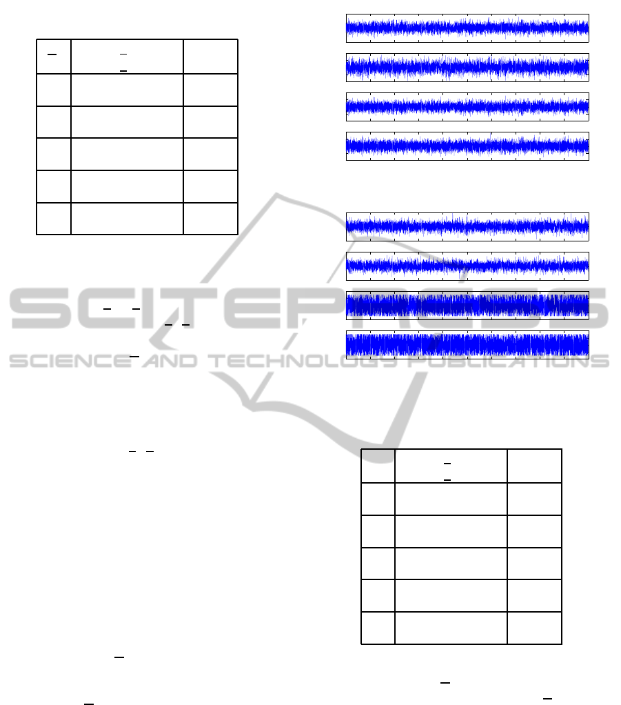
Table 1: Feedback gains and loss function values; failure
(3).
α
i
k
T
1
−
¯
α
i
k
T
2
¯
J
0.9 –0.9004, –0.3319 –
1.1 –0.1572, –1.0898 2.2794
0.7 –0.7492, –0.0924 –
1.3 0.0342, –0.7964 2.4626
0.5 –0.6357, 0.0989 –
1.5 0.1967, –0.5417 2.7634
0.3 –0.6141, 0.1750 –
1.7 0.3034, –0.3381 3.1764
0.1 –0.9880, 0.1943 –
1.9 0.5037, –0.2898 4.6344
Σ
w
=

1 0
0 1

,
Q = I, R = 0.1I and x
0
= 0.
The feedback gains K
T
= (k
1
, k
2
) and the corre-
sponding values of the loss function for few configu-
rations of system failure α
i
,
¯
α
i
are shown in Table 1.
The values of the loss function
¯
J were averaged over
10000 runs.
The feedback gains and the corresponding values
of the loss function for few constraints β
1
, β
2
for fail-
ure (23) are shown in Table 2. In this case, the sub-
optimal feedback gains k
1
, k
2
were calculated with
iterative procedure given in (Toivonen, 1983; Kro-
likowski, 2004) for given constraints β
1
, β
2
.
The optimal value of the loss function (also seen
from Table 2 for β
1
= β
2
= ∞) is J
opt
= 2.256. Fi-
nally, the feedback gains and the corresponding val-
ues of the loss function for failure (24) and different
constraints β
1
, β
2
are shown in Tables 3, 4, 5, 6. It
should be noticed that in this case the amplitude con-
straint β
i
in (24) is realized as a simple cut-off that
is obviously not an optimization approach like in the
previous case.
The exemplary run of inputs and outputs with ac-
tuator failure (3) with α
i
= 0.75,
¯
α
i
= 1.25, i = 1, 2
is shown in Fig.2 where the corresponding loss is
¯
J = 2.4018, and the corresponding run under actuator
failure (24) with α
i
= 0.75,
¯
α
i
= 1.25, β
i
= 1.5, i =
1, 2 is shown in Fig.3 where the corresponding loss is
¯
J = 2.5440.
Analyzing the values of the loss function given
in Tables 3, 4, 5, 6 one can observe a phenomenon
like the short-term behaviour phenomenon described
in (Chen et al., 1993; Chen et al., 1994) which takes
place when the minimum variance control is consid-
ered and the cutoff method is used to constrain the
control signal. This means that even though more
control effort is applied to the system, the closed-loop
system performance does not improve. The effect of
0 1000 2000 3000 4000 5000 6000 7000 8000 9000 10000
−5
0
5
x
1
0 1000 2000 3000 4000 5000 6000 7000 8000 9000 10000
−4
−2
0
2
4
x
2
0 1000 2000 3000 4000 5000 6000 7000 8000 9000 10000
−4
−2
0
2
4
u
1
0 1000 2000 3000 4000 5000 6000 7000 8000 9000 10000
−4
−2
0
2
4
u
2
k
Figure 2: Input and output signals for failure (3).
0 1000 2000 3000 4000 5000 6000 7000 8000 9000 10000
−5
0
5
x
1
(t)
0 1000 2000 3000 4000 5000 6000 7000 8000 9000 10000
−5
0
5
x
2
(t)
0 1000 2000 3000 4000 5000 6000 7000 8000 9000 10000
−2
−1
0
1
2
u
1
(t)
0 1000 2000 3000 4000 5000 6000 7000 8000 9000 10000
−2
−1
0
1
2
u
2
(t)
k
Figure 3: Input and output signals for failure (24).
Table 2: Feedback gains and loss function values; failure
(23).
β
1
k
T
1
−
β
2
k
T
2
¯
J
∞ –0.9322, –0.3821 –
∞ –0.1975, –1.1526 2.2567
1.5 –0.8594, –0.2113 –
1.5 –0.0544, –1.0186 2.4879
1.0 –0.7465, –0.0614 –
1.0 0.1423, –0.8302 2.7932
0.5 –0.5987, 0.1166 –
0.5 0.4141, –0.4282 4.3363
0.3 0.6192, 0.0785 –
0.3 0.5146, –0.2542 9.1401
that kind happens for α
i
= 0.0, 0.1,
¯
α
i
= 2.0, 1.9 as
illustrated in Fig.4, where the notation α
i
= 1 − δ,
¯
α
i
= 1 + δ is used. In Fig.5 where δ = 0.2, 0.3 the
effect is not seen. It can be concluded that the bigger
δ the stronger is the effect.
A similar phenomenon can be observed for given
β
i
and variable δ, for example for β
i
= 1.0, β
i
= 1.5
that is illustrated by Fig.6. Fig.7 shows the case β
i
=
0.3, β
i
= 0.5 where the effect is not seen.
DISCRETE-TIME LQG CONTROL WITH ACTUATOR FAILURE
519

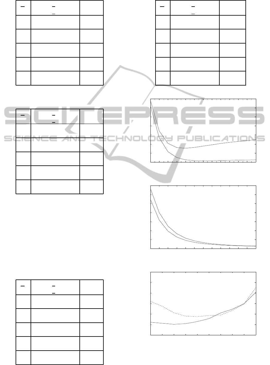
Table 3: Feedback gains and loss function values; failure
(24), β
1
= β
2
= 1.5.
α
i
k
T
1
−
¯
α
i
k
T
2
¯
J
0.9 –0.9004, –0.3319 –
1.1 –0.1572, –1.0898 2.5658
0.7 –0.7492, –0.0924 –
1.3 0.0342, –0.7964 2.5467
0.5 –0.6357, 0.0989 –
1.5 0.1967, –0.5417 2.7846
0.3 –0.6141, 0.1750 –
1.7 0.3034, –0.3381 3.1765
0.1 –0.9880, 0.1943 –
1.9 0.5037, –0.2898 4.2560
Table 4: Feedback gains and loss function values; failure
(24), β
1
= β
2
= 1.0.
α
i
k
T
1
−
¯
α
i
k
T
2
¯
J
0.9 –0.9004, –0.3319 –
1.1 –0.1572, –1.0898 3.3789
0.7 –0.7492, –0.0924 –
1.3 0.0342, –0.7964 2.9068
0.5 –0.6357, 0.0989 –
1.5 0.1967, –0.5417 2.9351
0.3 –0.6141, 0.1750 –
1.7 0.3034, –0.3381 3.2345
0.1 –0.9880, 0.1943 –
1.9 0.5037, –0.2898 4.0399
6 CONCLUSIONS
The problem of reliable LQG control for discrete-
time stochastic system is presented. An example of
a two-input system described by state-space equation
is taken for simulation. Simulation results show an
Table 5: Feedback gains and loss function values; failure
(24), β
1
= β
2
= 0.5.
α
i
k
T
1
−
¯
α
i
k
T
2
¯
J
0.9 –0.9004, –0.3319 –
1.1 –0.1572, –1.0898 8.7100
0.7 –0.7492, –0.0924 –
1.3 0.0342, –0.7964 5.8636
0.5 –0.6357, 0.0989 –
1.5 0.1967, –0.5417 5.0188
0.3 –0.6141, 0.1750 –
1.7 0.3034, –0.3381 4.8076
0.1 –0.9880, 0.1943 –
1.9 0.5037, –0.2898 4.9832
Table 6: Feedback gains and loss function values; failure
(24), β
1
= β
2
= 0.3.
α
i
k
T
1
−
¯
α
i
k
T
2
¯
J
0.9 –0.9004, –0.3319 –
1.1 –0.1572, –1.0898 18.3355
0.7 –0.7492, –0.0924 –
1.3 0.0342, –0.7964 12.9966
0.5 –0.6357, 0.0989 –
1.5 0.1967, –0.5417 11.3516
0.3 –0.6141, 0.1750 –
1.7 0.3034, –0.3381 10.7430
0.1 –0.9880, 0.1943 –
1.9 0.5037, –0.2898 10.2722
0.3 0.4 0.5 0.6 0.7 0.8 0.9 1 1.1 1.2 1.3 1.4 1.5
4
5
6
7
8
9
10
11
β
J
δ=1
δ=0.9
Figure 4: Loss function vs β for δ = 1.0, 0.9.
0,3 0,4 0,5 0,6 0,7 0,8 0,9 1 1,1 1,2 1,3 1,4 1,5
2
4
6
8
10
12
14
16
β
J
δ=0.2
δ=0.3
Figure 5: Loss function vs β for δ = 0.2, 0.3.
0 0.1 0.2 0.3 0.4 0.5 0.6 0.7 0.8 0.9
2
2.5
3
3.5
4
4.5
5
J
δ
β=1
β=1.5
Figure 6: Loss function vs δ for β = 1.0, 1.5.
ICINCO 2011 - 8th International Conference on Informatics in Control, Automation and Robotics
520

0 0.1 0.2 0.3 0.4 0.5 0.6 0.7 0.8 0.9
4
6
8
10
12
14
16
18
20
J
δ
β=0.3
β=0.5
Figure 7: Loss function vs δ for β = 0.3, 0.5.
effectivness of the proposed control algorithms as a
method for coping with actuator failure in the case of
state feedback LQG control. A failure in form of ac-
tuator saturation (23) has stronger impact on the loss
function than actuator failure given by (3), especially
for tight constraints. In that case the failure (24) has
even more stronger impact.
REFERENCES
Chen, G., Malik, O., and Hope, G. (1993). Control limits
consideration in discrete control system design. IEE
Proc.-D, 140(6):413–422.
Chen, G., Malik, O., and Hope, G. (1994). Generalised dis-
crete control system design method with control limit
considerations. IEE Proc.-D, 141(1):39–47.
Krolikowski, A. (2004). Adaptive control under input con-
straints (in Polish). Poznan University of Technology
Publisher.
Maciejowski, J. (2009). Fault-tolerant control - is it possi-
ble? In Diagnosis of Processes and Systems, pages
63–72. Pomeranian Science and Technology Publish-
ers PWNT.
Meier, L., Larson, R., and Tether, A. (1971). Dynamic pro-
gramming for stochastic control of discrete systems.
IEEE Trans. Automat. Contr., AC-10(6):767–775.
Toivonen, H. (1983). Multivariable controller for discrete
stochastic amplitude constrained systems. Modeling,
Identification and Control, 4(2):83–93.
Yang, G.-H., J.L., W., and Soh, Y. (2000a). Reliable lqg
control with sensor failure. IEE Proc.Control Theory
Appl., 147(4):433–439.
Yang, Y., Yang, G.-H., and Soh, Y. (2000b). Reliable con-
trol of discrete-time systems with actuator failure. IEE
Proc.Control Theory Appl., 147(4):428–432.
Zuo, Z., Ho, D., and Wang, Y. (2010). Fault tolerant con-
trol for singular systems with actuator saturation and
nonlinear perturbation. Automatica, 46:569–576.
DISCRETE-TIME LQG CONTROL WITH ACTUATOR FAILURE
521