SYNTHESIS OF THE SYSTEM FOR AUTOMATIC FORMATION
OF UNDERWATER VEHICLE’S PROGRAM VELOCITY
Vlsdimir Filaretov and Dmitry Yukhimets
Institute of Automatic and Control Processes, FEB RAS, Radio St. 10, Vladivostok, Russia
Keywords: Underwater vehicle, Spatial moving, Control system.
Abstract: In this paper a method of automatic formation of program signal of underwater vehicle’s (UV) movement is
proposed. This method allows providing its movement on desires spatial trajectory with maximal velocity
and desired accuracy. For this purpose an additional control loop is included in UV’s control system. This
control loop provides a tuning of UV’s desirable velocity of movement along desirable trajectory. If current
UV’s deviation from this trajectory more than allowable value then this control loop decreases a value of
UV’s desirable velocity and vice versa. Proposed approach provides to increase efficiency of using of
existing UV’s control systems.
1 INTRODUCTION
It has already created a lot of methods for synthesis
of high accuracy control systems (robust, self
adjustment est.) of underwater vehicle’s (UV)
movement on spatial trajectories (Yuh, 1995;
Fossen, 1994;
Antonelli, 2006 and est.). These
methods provide the high dynamic accuracy of
control. It is possible if UV’s actuators will be able
simultaneously to realize the UV’s moving program
signals and compensate the interactions between
different degrees of freedom. When UV is being
moved on trajectory’s parts with large curvature
some actuators will be able to reach of saturation. As
a result the UV will be able to deviate from desirable
trajectory.
It can eliminate this situation if it uses more
powerful actuators. But in this case the mass and
size of UV grows. Another decision it is moving
with small velocity which provides high accuracy of
UV’s movement along whole trajectory. But in this
case on the rectilinear parts of trajectory the UV will
be moves with velocity smaller then it possible.
So for more fully using of UV’s potential it is
necessary change of its velocity by dependence from
curvature of current trajectory’s part. On the part
with large curvature UV can significantly deviate
from desired trajectory and we must decrease
velocity. In this case the interaction between control
channels will be decreased and, consequently, the
level of control signals will be decreased too. On the
rectilinear parts of trajectory we can increase the
UV’s velocity, because in this case the interaction
between control channels are small.
The basic problem which arises during solving of
this task it is variability and uncertainty of UV’s
parameters during it moving in viscous environment
(Yuh, 1995); (Fossen, 1994); (
Antonelli, 2006);
(
Filaretov, 2006). Therefore it is possible to select a
UV’s motion mode only approximately. Also it is
ordinary situation when single actuator makes
control force for movement on several degrees of
freedom (Ageev, 2005). It is significantly
complicate selection of movement mode in cases
when movement takes place on several degrees of
freedom simultaneously.
In work (Lebedev, 2004) on the base of
kinematics equations the approach to automatic
formation of UV’s velocity was suggested. But this
approach not allows take into account the saturations
of actuators and dynamical properties of UV. In the
work (
Repoulias, 2005) the desirable mode of UV’s
movement is formed on the base equations of
dynamic and kinematics which describe work of UV
and it’s actuators complex. But in this work the
open-loop system is developed. This system not
provide accuracy UV’s movement.
In this paper the approach based on the automatic
formation of desirable UV’s velocity depending on
value its deviation from desirable trajectory is
offered. This approach not requires of identification
of UV’s parameters and has simple practical
realization.
439
Filaretov V. and Yukhimets D..
SYNTHESIS OF THE SYSTEM FOR AUTOMATIC FORMATION OF UNDERWATER VEHICLE’S PROGRAM VELOCITY.
DOI: 10.5220/0003644904390444
In Proceedings of the 8th International Conference on Informatics in Control, Automation and Robotics (MORAS-2011), pages 439-444
ISBN: 978-989-8425-75-1
Copyright
c
 2011 SCITEPRESS (Science and Technology Publications, Lda.)

2 PROBLEM DEFINITION
Let UV already have control system (CS)
))(*),(()( tXtFtu
u

 ,
(1)
where
n
Rtu )( is a vector of control signals of
UV’s actuators; n is a number of UV’s actuators;
3
)()(*)( RtXtXt   is a vector of UV’s
dynamical error;
3
))(*),(*),(*()(* RtztytxtX
T

and
3
))(),(),(()( RtztytxtX
T
 are vectors of
desirable and current UV’s position, respectively.
CS (1) provide for UV desirable control quality.
Let the desirable trajectory in Cartesian space is
described by following expressions:





*)(*
*)(*
xgz
xgy
z
y
(2)
In order to CS (1) provides the movement of UV
along trajectory (2), it is necessary to form vector
T
tztytxtX ))(*),(*),(*()(* 
. It gets more
comfortable to do if we set the desirable velocity
along trajectory (2). Vector
)(* tX
will be
calculated by formulas [6]:
*),(/)(*)(* xtvtx 

)),(*()(* txgty
y

))(*()(* txgtz
z
 ,
(3)
where )(* tv is a law of change UV’s desirable
velocity of movement on trajectory (2),
.
*
*)(
*
*)(
1*)(
2
2
















dx
xdg
dx
xdg
x
z
y
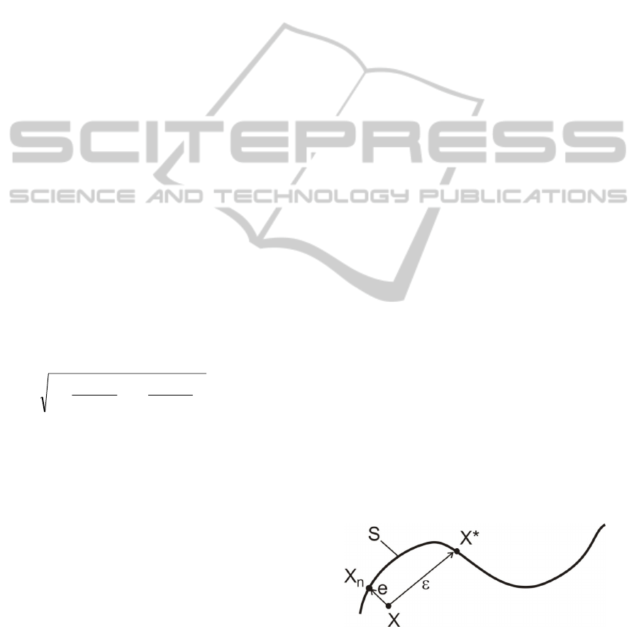
The dynamic error of tracing

t

arises at the
movement of UV with CS (1). Presence of


t

leads to deviation of UV from desirable trajectory
(2) on value
e(t) (see fig. 1). This deviation often is
most important characteristic of UV’s control
quality. The more trajectory’s part curvature is the
more value
e(t) is. It is obvious that for e(t) follow
condition is performed:
 
||||0 tte

 .
(4)
From inequality (4) it is clearly that for movement of
UV along desirable trajectory (2) with deviation

max
ete  ,
(5)
(where
max
e is a maximum allowed deviation of UV
from trajectory) is necessary restricts value
||||

.
Moreover (by dependence on current trajectory
curvature) the value
||||

can have different
restriction. The value
||||

on rectilinear parts of
trajectory for correctness of inequality (5) can be
more then the one on parts with large curvature. We
can restrict ||||

if we restrict speed of changing of
program signals or, according to expression (5),
UV’s desirable velocity. Regarding what is set
above in this work the following problem is set and
solved. Let UV include the CS (1). The vector of
program signals
)(* tX forms by expressions (3). It
is necessary create such law of change of UV’s
desirable velocity
)(* tv along trajectory (2) which
provides the correctness inequality (5).
3 DESCRIPTION OF SYSTEM
FOR FORMATION OF
PROGRAM SIGNALS OF
MOVEMENT
In this section we will considered the proposed
synthesis method of system for formation of UV’s
desirable velocity. This system must automatically
form a maximum possible value
)(* tv by
dependence on curvature of current trajectory’s part
and provide correctness of expression (5).
We could solve this task if we will get the
analytical expressions for formation of
)(* tv by
dependence on properties of UV and its trajectory.
But it is getting of these expressions practically
impossible because the mathematical model of UV
and it actuators complex is very complicated. So in
this work other approach proposes. It lies in creation
of addition control loop which automatically form
)(* tv by dependence on current deviation of UV
from desirable trajectory (2).
The general structure of proposed system is
shown on the figure 2.
Figure 1: The errors occurring at UV’s movement on
spatial trajectory.
ICINCO 2011 - 8th International Conference on Informatics in Control, Automation and Robotics
440

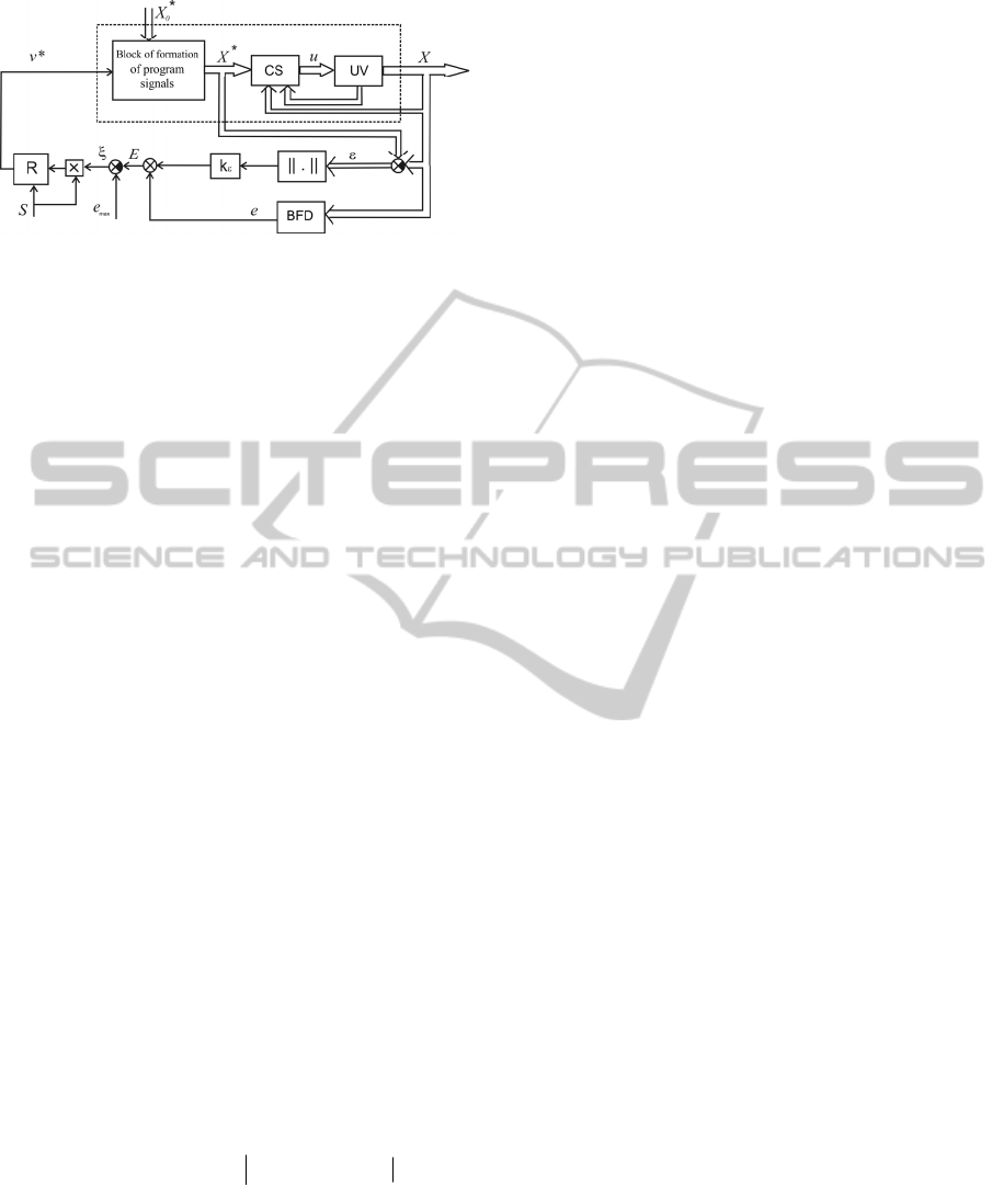
Figure 2: The block diagram of system for automatic
formation of UV’ desirable velocity.
In the beginning of work of this system the
signal
)(* tv is fed on the input of block of program
signals formation. On the output of this block the
vector of signals
T
tztytxtX ))(*),(*),(*()(* 
is
formed by expressions (3). This vector is fed on
input of UV’s CS which forms a control signals
)(tu for UV’s actuators (see expression (1)).
By using of current values of elements of vectors
)(and)(* tXtX the signal )(tE is formed:
  
tetktE
m



,
(6)
where
 
|||| tt
m


 ;

k = const is a positive
coefficient. Expression (6) defines accuracy of UV’s
movement on trajectory.
After the system (see fig. 2) is turned on the
regulator R form the signal
)(* tv by dependence on
current value
)(tE . Using this signal and expressions
(2) and (3) the vector
T
tztytxtX ))(*),(*),(*()(* 
is calculated. The work of system finish when UV
arrived to final point of trajectory. In this case the
signal
)(* tv is been set to zero by help of zero
signal
S (see fig. 2).
Value
e(t) in (6) is calculated as distance from
current UV’s position (vector
X) to nearest point on
desirable trajectory
X
n
),,(
nnn
zyx (see fig. 1) by
means of block of formation of deviation (BFD).
Coordinates of point
X
n
we can find as follows.
The vector

X of trajectory’s tangent line in
point
n
X has coordinates




T
xx
z
xx
ynv
n
n
dxxdgdxxdgxfX )*/*)(,*/*)(,1()(
*
*

T
nzny
xgxg ))(),(,1(


[8]. Vector which connect
points
X and
n
X perpendicular to vector

X .
Therefore the following equality is correctness:
0))((
))(()()(








zzxg
yyxgxxXXX
nnz
nnynn

.
(7)
Having solved the equation system (7) and (2),
we will be able to define coordinates of point
n
X .
Regulator R(
 ) is working as follows. If  (t) < 0,
then inequality e(t) >
max
e is correctness. In this case
regulator R(
 ) will be decreases )(* tv . It is going to
result in decreasing of value

|||| t

and in
accordance with (4) – to decreases of e(t). If
 (t) > 0,
then e(t) <
max
e and regulator R(  ) will be increases
)(* tv .
Notice that value
)(* tv must be nonnegative. It
is essentially important in the beginning of UV’s
movement when error between initial UV’s position
and initial point of trajectory may be large. In this
case nonnegativeness of
)(* tv allow to fix a
position of desirable point X* while UV come to it
on distance less then
max
e . Only after that the value
of
)(* tv begin to increase.
Also we have to restrict the value
)(* tv when
e(t) is small (for example when UV movement along
straight line). For this purpose we take into account
the value of


|||| t

at the formation of signal E(t)
(see expression (6)). First term in expression (6) will
be the main at the UV’s movement on the rectilinear
part of trajectory and second term will be the main at
one’s movement on the curvilinear part of trajectory.
In the next section we will considered a problem
of selection of regulator R (
).
4 THE SYNTHESIS OF UV’S
DESIRABLE VELOCITY
CONTROLLER
In the beginning we will get a mathematical model
of control object (CO) for regulator R. In this case
the signal v* is fed on the CO’s input and value E is
formed on the CO’s output by expression (6). This
CO include the block of formation of desirable
signals (3), UV’s CS and own UV (see fig. 2). It is
obvious that model of this CO is nonlinear.
Moreover a kind of trajectory is previously unknown
and it use of this model for synthesis of regulator
very difficult.
Therefore we will use the estimations of values E
and e instead their real values for simplification of
synthesis procedure. In this case the regulator R will
be synthesized independently on a kind of UV’s
trajectory and regulator’s structure simplify
significantly.
SYNTHESIS OF THE SYSTEM FOR AUTOMATIC FORMATION OF UNDERWATER VEHICLE'S PROGRAM
VELOCITY
441

First we estimate the value of E. Using the
inequality (4), we can write
me
ke

 ,
(8)
where 10 
e
k . Putting (9) in (6) we will get:
meme
kkkE 

~
)(  ,
(9)
where 1
~


kkk
e
.
The using of value
m

is going to result in big
difficulties at synthesis of regulator R. Therefore it
gets more comfortable to replace this value for value
||||||
~
zyxm




 , where
zyx



,, are
corresponding elements of vector
)(t

.
For this replacement we use fact that norms of
vector



n
i
i
aa
1
1
|||||| and
2/1
1
2
2
)||(||||



n
i
i
aa satisfy
following inequality (Korn, 1968):
2
2/1
12
|||||||||||| anaa  .
(10)
From expression (10) the justice of equality follows:
mmm
k


~
 ,
(11)
where
m
k is coefficient which satisfy the inequality
13/1 
m
k .
We suppose that using of CS (1) provides to
describe the UV’s dynamic to each degree of
freedom by transfer functions
),(sW
x
)(),( sWsW
zy
.
These transfer functions, written relatively errors,
have form:
).(1)(
),(1)(),(1)(
sWsW
sWsWsWsW
zz
yyxx




(12)
Therefore take into account of equality
aasigna )(||  and expressions (9)-(12) we can
write:
.
~
))(*)()()(*)(
))()(*)()(()(
emzzy
yxx
kkszsWsignsysW
signsxsWsignsE






(13)
If it supposes that )()()()( sWsWsWsW
zyx


then expression (13) take form:
))(*)()(*)(
)(*)()((
~
)(
szsignsysign
sxsignsWkksE
zy
xem





,
(14)
where )(1)( sWsW 

.
From expressions (3) it is simply to get:
).(*
*)(
*)(*
*
*)(
)(*
),(*
*)(
*)(
*
*
*)(
)(*
tv
x
xg
dt
dx
dx
xdg
tz
tv
x
xg
dt
dx
dx
xdg
ty
zz
yy








(15)
If we apply the Laplace transformation to expression
(15) then we get:
,/)(*)(*
,/)(*)(*,/)(*)(*
ssvksz
ssvksyssvksx
vz
vyvx



(16)
where
*)(/1 xk
vx

,


*),(/*/*)( xdxxdgk
yvy




*)(/*/*)( xdxxdgk
zvz


are current value of
corresponding functions.
Take into account (16) we can transform the
expression (14) to from:
).(*))()(
)((
)(
~
)(
svksignksign
ksign
s
sW
kksE
vzzvyy
vxxem





(17)
As CO (17) is inertial objects then point X* always
outstrip current UV’s position. So we can confirm
that signature of UV’s desirable velocity on
corresponding coordinate coincide with the signature
of dynamic error on this coordinate. It is aside from
small trajectory’s parts where the change of
signature of UV’s velocity on separate coordinates
takes place. The signature of dynamic error is
unequal to signature of desirable velocity on
corresponding coordinates on small time interval. So
in further reasoning we can ignore it phenomenon.
Regarding what is set above and
0*)(  x we
can present the penult multiplier in expression (17)
in form:
||||||
*
vzvyvxv
kkkk  .
(18)
We can see from expressions (3) and (16) that
equality
1)(
2/1
222

vzvyvxv
kkkk always will be
correct. Therefore take into account inequality (8) it
can write:
31
*

v
k .
(19)
As result the mathematical model of CO for
regulator R take into account expressions (17)-(19)
and entered assumptions can be presented in form:
ssvsWkkksE
emv
/)(*)(
~
)(
*

 ,
(20)
where 3)1(
~
3/3
*

kkkkk
vme
 .
Further we synthesize the regulator R for UV
which includes the CS discussed in work (Filaretov,
2006). This CS provides to describe a UV’s spatial
ICINCO 2011 - 8th International Conference on Informatics in Control, Automation and Robotics
442

movement on all translational degrees of freedom by
matrix differential equation:
** KXXCKXXCX 

.
(21)
where
3333
,

 RKRC
are diagonal matrices with
positive elements.
It is simply to get from equation (21) a transfer
function relatively error for each control channel of
UV’s translational movement:
kcssssW 
22
/)(

,
(22)
where
0
i
cc
,
0
i
kk
,
)3,1(i are elements
of matrices C and K respectively.
Take into account expressions (20) and (22) the
CO’s transfer function can be present as
 
)./(
~
/)(
2*
kcssskkkssEsW
vmep



(23)
It is obvious that transfer function of regulator R(s)
will has a form:
ssTksR
rr
/)1()(

 ,
(24)
then take into account expression (23) the transfer
function of open loop system will be in following:
kcss
sTkkkk
sWsRsW
rvmer
pr



2
*
)1(
~
)()()( .
(25)
As we can see from expression (25) the stability of
close loop system not depend from value of
coefficients
*
,,
~
,
vmer
kkkk . So parameters of
regulator R we can choose of any value by depend
on required characteristics of work quality.
5 THE SIMULATION OF WORK
OF SYNTHESIZED SYSTEM
The mathematical simulation for checking of
workability of synthesized system was carried out. It
supposes that UV already include the CS which
provides to describe of UV’s dynamic properties by
equation analogous the equation (20) (Filaretov,
2006). Therefore it supposes that UV has identical
actuators which are described as aperiodic links.
The UV’s mathematical model described in work
(Lebedev, 2004) was used during the simulation.
The CS’s parameters was selected so that the
elements of matrices C and K in equation (20) have
following values:
3,1,3.0,1  ick
ii
. The
parameters of regulator R(s) had values:
,10

r
k
,5.0 sT
r

,2.0


k
max
e = 0.2 m. During
simulation the UV’s horizontal movement along
trajectory


)20/*sin(10* txtz


. In this case it
supposes that
0
*
0
x , 0
*
0
z and UV’s long axis
always directed to point X* during UV’s movement.
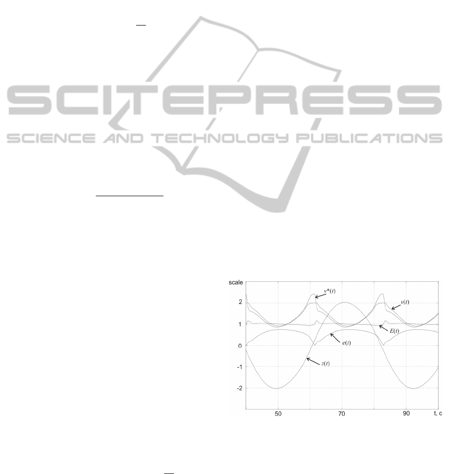
On the fig. 3 the processes of change of values
v*(t), v(t), е(t), Е(t) and z(t) during UV’s movement
on desired trajectory are shown.
On this figure we can see that minimal and
maximum value v*(t) is formed when UV move on
trajectory with minimal and maximum velocity
respectively (see curve z(t)). On the trajectories parts
which close to rectilinear е → 0, value v*(t)
increase, the UV’s actuators reaches to saturations
and value v(t) reaches to maximum. It is going to
result in fast increasing of
m

and E(t). As result
E(t) become more then e
max
and value v*(t) begin to
decrease. During the UV’s movement its desirable
velocity v*(t) changed from 0,85 m/s to 2,2 m/s and
real velocity v(t) from 0,9 m/s to 2 m/s.
For comparison on fig. 4 the simulation results is
shown for case of UV’s movement without using of
synthesized system of automatic formation of
desirable velocity.
In this case such value v*(t) = 0,9 m/s = const is
selected which provide correctness inequality
max
)( ete

on whole trajectory. On this figure we
can see that during UV’s movement with constant
value of v* the value of e less then 0,2 m too. But in
this case the UV spends for running of one period of
trajectory on 66 seconds and when the synthesized
system is used it spends only 45 seconds.
)(2.0)();(2.0)(
);(5)();/()();/()(*
мscaletEмscalete
мscaletzсмscaletvсмscaletv




Figure 3: Processes of change v*(t), z(t), e(t), E(t) when
the automatic system for formation of program signal of
UV’s movement is used.
SYNTHESIS OF THE SYSTEM FOR AUTOMATIC FORMATION OF UNDERWATER VEHICLE'S PROGRAM
VELOCITY
443

)/()(),/()(*);/()(
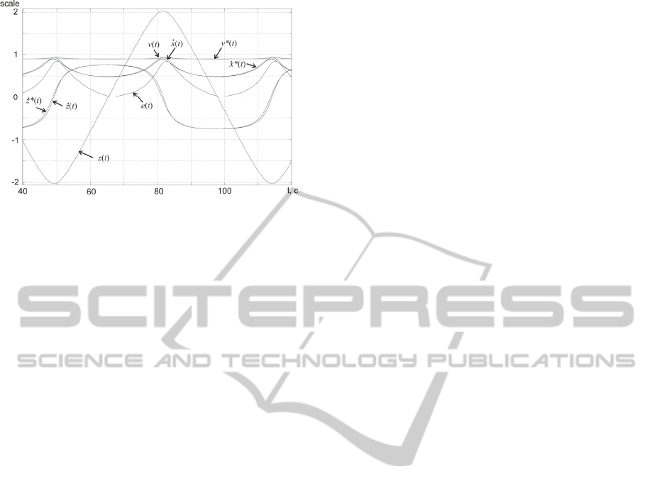
);/()(*);(2.0)(
);(5)();/()();/()(*
smscaletzsmscaletzsmscaletx
smscaletxmscalete
mscaletzsmscaletvsmscaletv







Figure 4: UV’s movement without using of automatic
system for formation of program signals.
Thus the simulation results confirm the
workability of synthesized system for automatic
formation of UV’s desirable velocity.
6 CONCLUSIONS
Thus in this paper the new method for formation of
UV’s program signals is suggested. This method
allow automatically set such UV’s desirable velocity
which provide UV’s movement on desirable
trajectory with deviation less then allowable value.
The formation of this desirable velocity takes place
by using of current deviation of UV from desirable
trajectory and norm of dynamic error vector. In this
work the block diagram of this system was
suggested and the selection of desirable velocity
regulator was proved. It has carried out the
mathematical simulation which shows the
workability and efficiently suggested approach.
ACKNOWLEDGEMENTS
This work is supported by Russian foundation for
basic research (grants #09-08-00080 and #10-07-
00395).
REFERENCES
Yuh J., (Editor), 1995. Underwater Robotic Vehicles:
Design and Control. TSI Press.
Fossen T. I., 1994. Guidance and Control of Ocean
Vehicles. John Wiley And Sons, New York.
Antonelli G., 2006. Underwater Robots. Springer Verlag.
Filaretov V. F., Yukhimets D. A., 2006. Design of
Adaptive Control System for Autonomous Underwater
Vehicle Spatial Motion. In Proc. of the 6th Asian
Control Conference. Bali, Indonesia, pp.900-906.
Ageev M. D., Kiselev L. V., Matvienko Yu, V., 2005.
Autonomous underwater robots: system and
technology. Nauka, Moscow. (in Russian)
Lebedev A. V., 2004. Synthesis of algorithm and the
device of formation of a trajectory of movement of
dynamic object taking into account restrictions on
operating signals. In Proc. of the IX Int. Chitaev conf.
“Analitical mechanic, stability and motion control”,
Irkutsk, Russia, Vol. 4, pp. 137-145. (in Russian)
Repoulias F., Papadopoulos E., 2005. On spatial trajectory
planning & open-loop control for underactuated
AUVs. In Proc of the 16th IFAC World Congress,
Prague, Czech Rep.
Korn G., Korn M., 1968. Mathematical handbook for
scientists and engineers. McGraw Hill Book
Company.
ICINCO 2011 - 8th International Conference on Informatics in Control, Automation and Robotics
444