
INVERSE METHOD FOR THE RETRIEVAL OF OCEAN
VERTICAL PROFILES USING SELF ORGANIZING
MAPS AND HIDDEN MARKOV MODELS
Application on Ocean Colour Satellite Image Inversion
Charantonis Anastase Alexandre
1
, Brajard Julien
1
, Moulin Cyril
2
, Bardan Fouad
3
and Thiria Sylvie
1
1
Laboratoire d’Océanographie Climat et Analyses Numériques, Université Pierre et Marrie Curie
Tour 45-55, 4, Place Jussieu, 75252, Paris, France
2
Laboratoire des Sciences du Climat et de l'Environnement, L'Orme des Merisiers, CEA Saclay
bat 712, 91191, Gif-sur-Yvette, France
3
Laboratoire CEDRIC, Conservatoir National des Arts et Metiers (CNAM), 292, Rue Saint Martin, 75003, Paris, France
Keywords: Self organising maps, Hidden markov models, Inversion, Geophysical, Chlorophyll-A, Satellite imaging,
Inversion.
Abstract: This paper presents a statistical inversion method used to infer 3D data from 2D imaging. The methodology
is based on a combination of the Self Organising Maps and the Hidden Markov Models. The method has
been validated by inferring the oceanic vertical profiles of Chlorophyll-A based on sea-surface data.
1 INTRODUCTION
The density of satellite observations allowed a semi-
continuous observation of the global ocean surface.
The two-dimensional images provided by this
coverage often contain information on integrated
quantities whose vertical distribution is unknown.
Depending on the field of study there exist different
dynamic approaches for inverting this type of data.
However, these approaches are often faced with the
problem of non-linearity, and can also be hampered
by a lack of knowledge of the complete mechanisms
that govern the distributions.
The present paper deals with the inversion of
observed sea-surface satellite images, noted
∈
1⋯
, for retrieving of the vertical distribution
of Chlorophyll-A, noted
∈
1⋯
, using a
statistical, non-linear approach.
The methodology we have developed is a
mixture of the neuronal algorithms known as Self
Organizing Topological Maps (SOM) and the
Hidden Markov Models (HMM). The SOM are
unsupervised classification algorithms, that allow us
to cluster our availiable data into classes. The classes
are arranged on a topological map and connected to
each other by a topological similarity distance. In the
present study the SOM classification is applied
twice, once on the sea-surface data, and once upon
the vertical profiles connected to these images. The
resulting topological maps allow us to discretize
both data spaces into set amounts of classes.
The second statistical algorithm, the HMM
allows us to infer the most likely sequence of some
discrete, unobservable states, given a series of
discrete, observable states. To do so a set of
probability matrices are calculated, corresponding to
the dynamic processes of the unobserved states and
the links existing between the observed and
unobserved states. We use the classes created
through the SOMs to discretize the availiable data
and therefore represent both the observable and the
unobservable states.
In this paper, we present the results obtained
with the methodology developed on a case study at
the site of the Bermuda Atlantic Time Series
(BATS) (32 N -64 W) of the JGOFS campaign.
2 SELF-ORGANIZING
TOPOLOGICAL MAPS
Self-Organising Topological Maps (SOM) are
316
Anastase Alexandre C., Julien B., Cyril M., Fouad B. and Sylvie T..
INVERSE METHOD FOR THE RETRIEVAL OF OCEAN VERTICAL PROFILES USING SELF ORGANIZING MAPS AND HIDDEN MARKOV MODELS
- Application on Ocean Colour Satellite Image Inversion.
DOI: 10.5220/0003644703160321
In Proceedings of the International Conference on Neural Computation Theory and Applications (NCTA-2011), pages 316-321
ISBN: 978-989-8425-84-3
Copyright
c
2011 SCITEPRESS (Science and Technology Publications, Lda.)
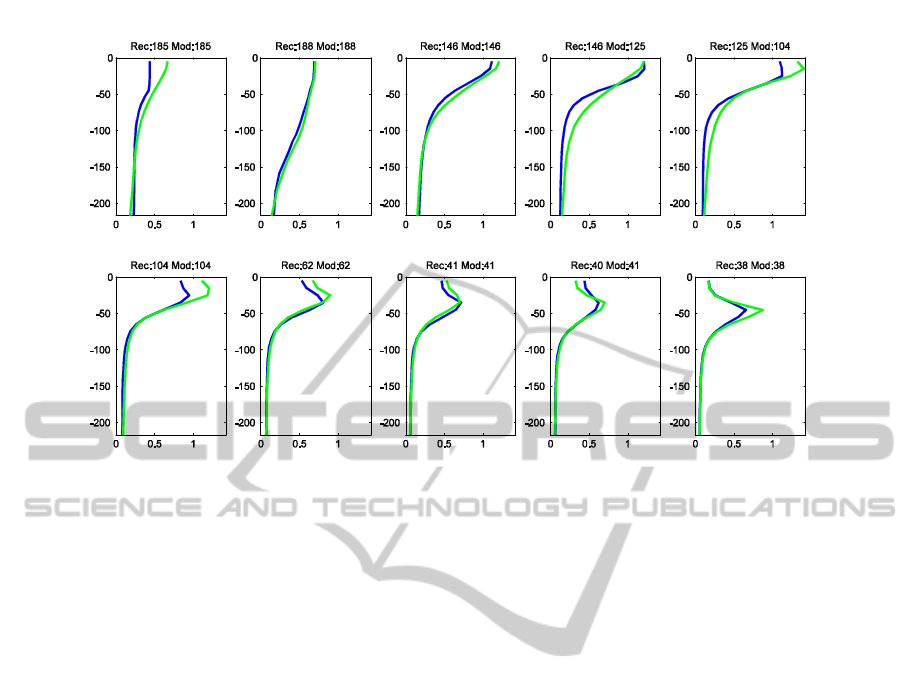
Figure 1: Inversion of ten 5-days steps for the period from 04-04-2005 to 05-19-2005, at BATS. In green, the states
provided by the inverse method and in blue the vertical distribution of Chlorophyll-A according to the NEMO-PISCES
model. The horizontal axes are in 10
6
μmol/L of Chlorophyll-A, while the vertical ones are in meters from the sea surface.
The numbers on top correspond, after Rec, to the indexes of the classes on M
dis
attributed to that 5-day step by the inverse
method, and, after Mo to the indexes attributed by projection of the total profile on M
dis
. These are not show in the figure.
clustering methods based on neural networks (S,
Haykin 1999). They provide a discretization of a
learning dataset A= {
∈
, k =1...N } into a
reduced number of subsets, called classes, P
i
, { i =
1...M } that share some common statistical
characteristics. Each subset is represented by its
referent vector r
i
which approaches the mean value
of the elements in the class Pi. In our case, we
trained two SOMs, one containing the observations,
called M
obs
and one containing the distributions of
the unobservable states, called M
dis
. The number of
classes in M
obs
and M
dis
are respectively noted N
obs
and N
dis
.
The topological aspect of the maps can be
justified if we consider the Map as an undirected
graph on a two-dimensional lattice whose vertices
are the m classes. This graph structure therefore
allows the definition of an discrete distance d(i,j)
between two classes i and j, defined as the length of
the shortest path between i and j on the map. The
nature of the SOM training algorithm forces a
topological ordering upon the map, and therefore
any neighbouring classes c
i
and c
j
on the map have
referent vectors r
i
and r
j
that are close in the
Euclidian sense in the data space R
P
.The topological
ordering constitutes a major element of our inverse
method, since it allows us to make, latter on, the
ergodic assumption for our Markov states.
We define a series of observable events by taking
the data from observations related to a given period
of time and we label each observation by the index
of the class to which it is assigned by using M
obs
.
This classification is done by allocating to each
observation
∈
1⋯
, in the sequence the
index of the class of M
obs
whose referent is the
closest to it in the Euclidian sense. Therefore we
obtain the series
S
obs
=
=
−
,
=1⋯
(1)
In the same way, we obtain the time-series of
distributions
S
dis
=
=
−
, =
1⋯
(2)
These series S
obs
and S
dis
are used by the HMM in
order to estimate the probabilistic links that exist
between the observable states and the unobservable
ones.
The referents r
dis
of M
dis
are also used as the
vertical profiles in our sequence reconstructions.
04-04-2005 09-04-2005 14-04-2005 19-04-2005 24-04-2005
29-04-2005 04-05-2005 09-05-2005 14-05-2005 19-05-2005
INVERSE METHOD FOR THE RETRIEVAL OF OCEAN VERTICAL PROFILES USING SELF ORGANIZING MAPS
AND HIDDEN MARKOV MODELS - Application on Ocean Colour Satellite Image Inversion
317
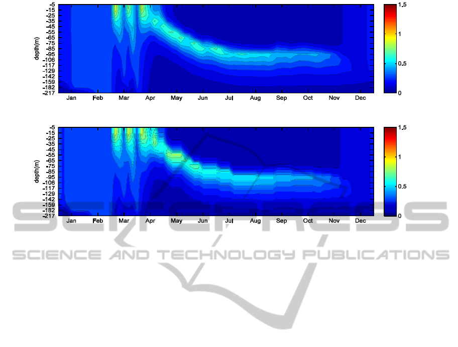
Figure 2: The reconstruction at BATS of the validation year 2005, according to, the NEMO-PISCES MODEL (top graph)
and the inverse method result (bottom graph). The colorbar indicates the Chlorophyll-A concentration in 10
6
μmol/L.
3 HIDDEN MARKOV MODELS
A Markov model is a stochastic model that assumes
the first order Markovian property, meaning that
each consecutive state of the model depends solely
on its previous stat of the model such as
P(X
t
| X
1
X
2
... X
t-1
) = P(X
t
| X
t-1
) (3)
Expanding this principle, a Hidden Markov Model
(HMM) is a stochastic model with two sequences.
One sequence of unobservable states that follow the
first order Markovian property, (represented in our
method by S
dis
), and one sequence of observable
states, (represented by S
obs
), that have a statistical
link with the unobservable states (O. Cappé et al.,
2005).
We consider two phases, a training one, and a
retrieval one. During the training, the Transitions
matrix Tr and the Emissions matrix Em are
estimated. Tr contains the transition probabilities of
the unobserved states
tr
i,j
= P(C
dis(i,t)
| C
dis(j,t-1)
) (4)
where
∑
,
=1
(5)
Tr corresponds, in a physical sense, to the
underlying dynamics that govern the unobserved
states.
Em contains the à posteriori probabilities of
each observed state to have been emitted by an
unobserved state,
e
i,j
= P(C
dis(i,t)
| C
obs(j,t)
)
(6)
where
∑
,
=1
(7)
Em corresponds, in a physical sense, to the link
existing between the observed quantities and the
dynamics of the unobserved quantities. Another
probability matrix that needs to be calculated is the
initial probability matrix Π, with components π
i
which represent the average revisit rate of each
unobserved state given an infinite sequence. All
mentioned probabilities are estimated by using the
Baum-Weltch algorithm (L. E. Baum et al., 1970),
which is a maximum likelihood optimization
algorithm, that takes as input the sequences S
obs
and
S
dis
and outputs the most likely matrices to have
generated them through a hidden Markov process.
During the recognition phase, we used the
Viterbi algorithm, which is a well-know dynamic
programming algorithm (Viterbi AJ, 1967), for
inferring the most likely sequence of indexes S
dis-est
representing the unobserved states, given the
previously estimated parameters Tr, Em and Π of the
HMM and a sequence of observations S
obs-new
. It is
well documented (M.S. Ryan and G.R. Nudd. 1993)
that the Viterbi algorithm can face problems due to
NCTA 2011 - International Conference on Neural Computation Theory and Applications
318
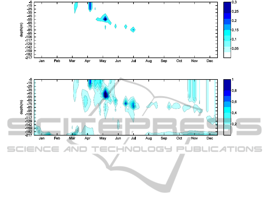
Figure 3: The top image contains the absolute error between the NEMO-PISCES model and the result of the inverse
method, at BATS for the validation year 2005. The bottom image contains the absolute relative error between the NEMO-
PISCES model and the result of the inverse method.
transitions that were not observed in the training
data set. A balance needs to be found between the
sizes of the SOM maps that will determine the
amount of discretization provided by the method,
and the correctness of the allocation of indices. The
dimensions of each map are therefore optimized
using a validation set. Yet, even with an
optimization there will be some situations and
transitions that are seldomly encountered in the
training data and result in null probabilities in the
probability matrices Em
B-W
and Tr
B-W
that we
estimated in the first pass of the Baum-Weltch
algorithm.
Due to this usual lack of sufficient data in the
concerned domains, Em
B-W
and Tr
B-W
need to be
adjusted. This is done by taking into account the
properties of the topological maps. A major
characteristic of the present method is to use the
topological order in order to improve the accuracy of
the estimated probabilities matrices. The topological
maps allow us to modify the probabilities by
allowing each state to communicate via a diminutive
probability with each of its neighbouring states.
This is done by considering the neighbourhood
matrices NM
obs
and NM
dis
, of dimensions (N
obs
,N
obs
)
and (N
dis
,N
dis
), where
NM
SOM
(i,j)=
1,i
f
d
,
<2
0,
(8)
with d(i,j) being the discrete distance of the map.
Taking into account the neighbourhood consists in
increasing the probability of reaching a class j from
a class i, by an ammount proportional to the sum of
the previously calculated probabilities of reaching
the neighbour classes of class j on SOM. In order to
favour the data observed during training, we add a
weighting term, noted w
c
, to the initial probabilities,
and we further multiply it by the total length of the
training sequences used in the intitial Baum-Weltch
algorithm’s pass, noted T
training
, since this length is a
measure of confidence in the correctness of the
estimated parameters. The matrices obtained are
then normalized. The final Em and Tr matrices we
use, noted Em
final
and Tr
final
, are computed by
applying:
,
=
∗
∗
,
+
∑
,
∗
,
+1
(9)
Which is normalized to fit the constraint (7), and
,
=
∗
∗
,
+
∑
,
∗
,
(10)
Which is normalized to fit the constraint (5). For this
application w
c
is set to 9.
INVERSE METHOD FOR THE RETRIEVAL OF OCEAN VERTICAL PROFILES USING SELF ORGANIZING MAPS
AND HIDDEN MARKOV MODELS - Application on Ocean Colour Satellite Image Inversion
319

These modifications permit the Viterbi algorithm
to circumvent the problems of impossible
transitions, or emissions due to insufficient data in
the training sequences that resulted in nul
probabilities in the estimated parameters.
4 APPLICATION FOR THE
RESTITUTION OF THE
VERTICAL CHLOROPHYLL-
A CONCENTRATION
THROUGH SEA SURFACE
DATA
The bio-geochemical activity of the oceans and the
carbon cycle are two parts of a complex feedback
system. A change in climate and an increase of the
amount of available carbon can affect the primary
oceanic production, and in return a change in the
bio-geochemical activity affects, by modifying the
albedo and carbon fixation rates, the climate and
carbon concentration. It is therefore important to be
able to determine the oceanic primary production. In
recent years, many algorithms have been developed
that infer the Chlorophyll-A concentration in ocean
surface layers through satellite imaging (Brajard et
al., 2008). It has also been proved that the vertical
Chlorophyll-A distribution, is correlated with sea
surface data (Uitz et al., 2006). Therefore, the
determination of the vertical distribution of
Chlorophyll-A from sea surface data is a problem
that can be solved by the methodology we propose.
One cannot determine the vertical distribution of
Chlorophyll-A without first understanding the
parameters that influence the development of
phytoplankton. It is generally accepted that
phytoplankton growth depends on 5 parameters:
available radiation, available nutriments, predators
and biology, water temperature, water turbidity.
These parameters cannot easily be monitored
through a direct approach. Satellite imaging,
however, can give us proxy information, which can
be used in an empirical approach for determining the
vertical distribution of Chlorophyll-A. Specifically,
in this study we used: Sea Surface Chlorophyll-A
concentration (SCHL), Sea Surface Temperature
(SST), Sea Surface Elevation (SSH), Shortwave
Radiation (SR) and Wind-speed Intensity (WS).
Since our objective is to validate the theoretical
methodology, we used simulated data in order to test
the validity of our approach. We therefore
approximated the satellite values of the previous
parameters by using the input and output values
provided by the NEMO oceanic circulation model
coupled to the PISCES bio-geochemical model (C.
Moulin, 2008). In order to better simulate the noise
and errors inherent to satellite images we added a
white noise z ~ N(0,ê), ê=1/2 * (σ
schl
, σ
sst
, σ
ssh
, σ
ws
,
σ
sr
) to the parameters that could be gathered from
satellite imaging. σ represents the standard
derivation of each corresponding surface parameter,
as computed on the training data. The application
was set at the site of BATS.
The unobserved states that were classified, were
the output data vectors containing the average
vertical Chlorophyll-A distribution at 17 depth
levels (from 5 meters to 217) and temperature
distribution at 9 depth levels. These vertical
distribution profiles were 5-day averages spanning
the period from 1991 to 2007 located in a 2°x2°
square centred on BATS. Therefore M
dis
belongs to
R
26
(17 levels of Chlorophyll-A + 9 levels of
Temperature). M
obs
belongs to R
5
.
We trained M
obs
and M
dis
by taking into account
all available profiles at BATS, as well as any
adjacent points included in the model. This gave us
9*73*17=11169 profiles for the construction of the
maps. The optimum map sizes, N
obs
and N
dis
were
determined to be 21*14=294 classes.
For the estimation of the HHM parameters on
the other hand, we take a total of 14 years (1991-
2004) for the training, each including seventy-three
5-day steps. Therefore T
training
=1022. We maintained
3 years (2005-2007), or 219 5-day steps, to validate
our approach.
The results shown in Figure 1 present the
temporary evolution of Chlorophyll-A profiles in ten
5-day steps sequence, from 04-04-2005 to 19-05-
2005, at BATS. In green we see the Chlorophyll-A
distribution profiles, taken from the referents r
dis
of
M
dis
, corresponding to the indexes of the
reconstructed time series S
dis-rec
. In blue we can see
the vertical distribution of Chlorophyll-A according
to the NEMO-PISCES model at the same 5-day
steps.
In Figure 1 we also have, preceded by the
acronym Rec, the indexes that constitute time series
S
dis-rec
and, preceeded by Mod, the indexes we obtain
by projecting the corresponding profiles of the
NEMO-PISCES model on M
dis
. In order to avoid
confusion, the profiles corresponding to the indexes
after Mod are not displayed. When the vertical
distribution of Chlorophyll-A is know, these indexes
would correspond to the optimum reconstruction we
could get with M
dis
. We note this optimum time
series as S
dis-opt
. It is interesting to notice that even
NCTA 2011 - International Conference on Neural Computation Theory and Applications
320

when the indexes are not equal, the classes are
neighbours on M
dis
, and the estimated profiles are
quite similar to the observed ones.
If we define S
dis-2005to2007
as the reconstructed
time series of indexes of the validation years from
2005 to 2007 and as S
dis-opt-2005to2007
the
corresponding optimum reconstruction we observe
that they are in agreement 84,59% of the time. This
perforance reaches 88,58% when applied on the
reconstruction S
dis-2005
of the year 2005 alone, as
compared to its optimum reconstruction. This was
probably due to the validation year 2005 having a
small variation from the mean year, and presenting
often-observed transitions. In the training date we
had on average an agreement of 86,46%
In Figures 2 and 3, we applied the inverse
method to the full 73 5-day steps serie of the
validation year 2005. We can observe that the
reconstruction closely fits the results provided by the
NEMO-PISCES model. The correlation index of the
two images in Figure 2 is 97,30%.
We can notice that the discretization induced by
the SOM is apparent, yet the general form and
intensity are correctly represented, as it becomes
clear in Figure 3, where the error graphs tend to have
small values.
5 CONCLUSIONS
In the present paper we have introduced an inversion
method based on SOM and HMM, that is able to
reconstruct the vertical profiles of Chlorophyll-A
based on satellite images. One of its main
advantages in the inversion of Chlrophyll-A is that it
does not use Gaussian approxiamtions used in other
methods (Morel 1988, Uitz et al., 2006), allowing
the reconstruction of situations where the
distribution is not conforming to a single gaussian
curve. An additional benefit of the inversion method
presented, is its efficiency in terms of calculations.
The method is open ended enough to be applicable
for the inversion of the profiles of different bio-
geophysical parameters based on satellite imaging.
We plan to further validate this method by
testing its robustness with satellite imaging and in-
situ data, as well as to apply it on different types of
profiles, such as oceanic salinity or temperature
profiles. A latter goal is to expand the method to
take spatial constraints into consideration, and
reconstruct 3D profiles.
ACKNOWLEDGEMENTS
We would like to thank the “Délégation Generale de
l’Armement” for financing this work.
REFERENCES
S, Haykin 1999. "9. Self-organizing maps". Neural
networks - A comprehensive foundation (2nd ed.).
Prentice-Hall
L. E. Baum, T. Petrie, G. Soules, and N. Weiss, 1970. "A
maximization technique occurring in the statistical
analysis of probabilistic functions of Markov chains",
Ann. Math. Statist., vol. 41, no. 1, pp. 164–171.
F. Badran, M. Berrada, J. Brajarda M. Crépon,C. Sorror,
S. Thiria, J.-P. Hermand M. Meyer, L. Perichob and
M. Asch, 2008. "Inversion of satellite ocean colour
imagery and geoacoustic characterization of seabed
properties: Variational data inversion using a semi-
automatic adjoint approach", Journal of Marine
Systems, Volume 69, Issues 1-2, Pages 126-136
C. Moulin, A. Kremeur, A. El Moussaoui, C. Ethe, L.
Bopp, E. Dombrowsky, E. Greiner, O. Aumont, P.
Brasseur, 2008. "Understanding the interannual
variability of the oceanic carbon cycle: Results from
the coupled biogeochemical-physical global model
PISCES-NEMO", American Geophysical Union, Fall
Meeting 2008, abstract #OS31A-1226 Journal of
Marine Systems,Volume 69, Issues 1-2, Pages 126-136
J. Uitz, H. Claustre, A. Morel, S. B. Hooker, 2006
"Vertical distribution of phytoplankton communities in
open ocean: An assessment based on surface
chlorophyll", Journal of Geophysical Research
Vol.111.
Olivier Cappé, Eric Moulines, and Tobias Rydén, 2005.
"Inference in Hidden Markov Models." Springer.
Viterbi A J, 1967. "Error bounds for convolutional codes
and an asymptotically optimum decoding algorithm".
IEEE Transactions on Information Theory 13 (2):
260–269.
M. S. Ryan and G. R. Nudd. 1993. The Viterbi Algorithm.
Technical Report University of Warwick RR-238
INVERSE METHOD FOR THE RETRIEVAL OF OCEAN VERTICAL PROFILES USING SELF ORGANIZING MAPS
AND HIDDEN MARKOV MODELS - Application on Ocean Colour Satellite Image Inversion
321
