
SEGMENTED–MEMORY RECURRENT NEURAL NETWORKS
VERSUS HIDDEN MARKOV MODELS IN EMOTION
RECOGNITION FROM SPEECH
Stefan Gl¨uge, Ronald B¨ock and Andreas Wendemuth
Faculty of Electrical Engineering and Information Technology, Otto von Guericke University Magdeburg
Universit¨atsplatz 2, 39106 Magdeburg, Germany
Keywords:
Segmented-memory recurrent neural networks, Emotion recognition from speech.
Abstract:
Emotion recognition from speech means to determine the emotional state of a speaker from his or her voice.
Today’s most used classifiers in this field are Hidden Markov Models (HMMs) and Support Vector Machines.
Both architectures are not made to consider the full dynamic character of speech. However, HMMs are able
to capture the temporal characteristics of speech on phoneme, word, or utterance level but fail to learn the
dynamics of the input signal on short time scales (e.g., frame rate). The use of dynamical features (first and
second derivatives of speech features) attenuates this problem. We propose the use of Segmented-Memory
Recurrent Neural Networks to learn the full spectrum of speech dynamics.
Therefore, the dynamical features can be removed form the input data. The resulting neural network classifier
is compared to HMMs that use the reduced feature set as well as to HMMs that work with the full set of
features. The networks perform comparable to HMMs while using significantly less features.
1 INTRODUCTION
Automatic emotion recognition from speech aims at
identifying the emotional or physical state of a human
being from his or her voice (Ververidis and Kotropou-
los, 2006). The motivation for it mainly arises from
the wish for a natural man-machine interaction. De-
termination of the emotional state of a user helps to
derive the semantics of a spoken sentence and fur-
ther enables the machine to respond in an appropriate
manner, for example to adapt the dialogue strategy
(Vlasenko and Wendemuth, 2009a). Further, there is
a number of possible applications in various fields,
for instance, in the in-car environment to monitor the
emotional state of the driver (Schuller et al., 2004), in
call centres to detect angry speech (Kim and Hansen,
2010), and in psychology to support the diagnosis
of psychiatric disorders (Yingthawornsuk and Shiavi,
2008).
Emotion recognition from speech means to extract
adequate features from raw speech data followed by
the classification of the feature-representation of an
utterance. In many cases, utterances are labelled with
basic emotions like anger, boredom, disgust, etc. (Ek-
man, 1992). Furthermore, utterances can be classi-
fied as a point in emotion space with the dimensions
valance-arousal-dominance (Grimm et al., 2007) or
pleasure-arousal-dominance (Mehrabian, 1996). Yet,
a large range of classifiers was used for speech emo-
tion recognition. First of all, Hidden Markov Mod-
els (HMMs) represent a standard practice (Nwe et al.,
2003; Song et al., 2008; Inoue et al., 2011). El Ayadi
et al., 2011 state:
“Based on several studies (...), we can conclude
that HMM is the most used classifier in emotion clas-
sification probably because it is widely used in almost
all speech applications.”
Beside HMM, Support Vector Machines have
been used (Pierre-Yves, 2003; Schuller et al., 2009b),
and different kinds of neural networks. For in-
stance, feedforward networks (Nicholson et al., 1999;
Petrushin, 2000), Long Short-Term Memory Recur-
rent Neural Networks (W¨ollmer et al., 2008) and
Echo State Networks (Scherer et al., 2008; Trentin
et al., 2010).
In this work we use a novel recurrent network ar-
chitecture called Segmented-Memory Recurrent Neu-
ral Network (SMRNN) (Chen and Chaudhari, 2009)
to solve the task of emotion classification from
speech. Those networks are able to learn long-term
and short-term time dependencies in the input data.
By that, we can waive the dynamic features of the in-
308
Glüge S., Böck R. and Wendemuth A..
SEGMENTED–MEMORY RECURRENT NEURAL NETWORKS VERSUS HIDDEN MARKOV MODELS IN EMOTION RECOGNITION FROM SPEECH.
DOI: 10.5220/0003644003080315
In Proceedings of the International Conference on Neural Computation Theory and Applications (NCTA-2011), pages 308-315
ISBN: 978-989-8425-84-3
Copyright
c
2011 SCITEPRESS (Science and Technology Publications, Lda.)
S
0
S
1
a
01
a
11
a
02
b
0
(o
0
)
b
1
(o
1
)
S
i
S
j
a
ij
a
jj
a
ik
b
i
(o
i
)
b
j
(o
j
)
S
k
a
kk
b
k
(o
k
)
a
jk
a
ii
...
...
Figure 1: HMM topology.
put data, that is, reduce the feature set. The results
are compared to HMM classifiers that work with the
reduced feature set (no dynamic features) and the full
set of features.
The paper is organised as follows. Section 2 re-
veals the basic concept of HMMs and SMRNNs. Sec-
tion 3 introduces the speech database, feature extrac-
tion from the speech signal, and configuration of the
HMM and SMRNN classifiers. The results are pre-
sented in Sec. 4 and discussed in Sec. 5.
2 METHODS
2.1 Hidden Markov Models
The principle of the HMM is based on the Markov
characteristic of a process, i.e., the successive pro-
cessing step is independent from previous decisions
(Rabiner and Juang, 1993; Tuzlukov, 2000). Gen-
erally, HMMs are powerful in signal processing
(Boreczky and Wilcox, 1998; Schmidt et al., 2010) as
well as in speech processing and recognition (Rabiner
and Juang, 1993; El Ayadi et al., 2011). Such a model
is a finite state automata, which passes from state s
i
to state s
j
in each time slot, where i and j are ele-
ments of the state number set. Traversing the model,
an observation sequence o
i
is produced according to
a probability density b
i
(o
i
). Also the hidden values
a
ij
are probabilistic, representing the transition like-
lihood from state s
i
to s
j
. A visualisation is given in
Fig. 1.
The training process of HMMs is done by the
Baum-Welsh-Algorithm (Baum et al., 1970) and the
most likely observation sequence is computed by the
Viterbi-Algorithm (Viterbi, 1967).
2.2 Segmented-memory Recurrent
Neural Networks
Conventional Recurrent Neural Networks (RNNs)
suffer the vanishing gradient problem (Bengio et al.,
1994; Hochreiter, 1998) in learning long-term de-
pendencies. The Segmented-Memory Recurrent Neu-
ral Network architecture, recently proposed by (Chen
and Chaudhari, 2009), approaches the problem based
on the observation on human memorization. Dur-
ing the process of memorization of long sequences,
it is widely recognised that people fractionise it into
segments. In the end, the single segments are con-
nected in series and form the final sequence (Severin
and Rigby, 1963; Hitch et al., 1996). For instance,
telephone numbers are often broken into segments of
two or three digits to ease the memorization such that
6718959 becomes 67 - 18 - 959.
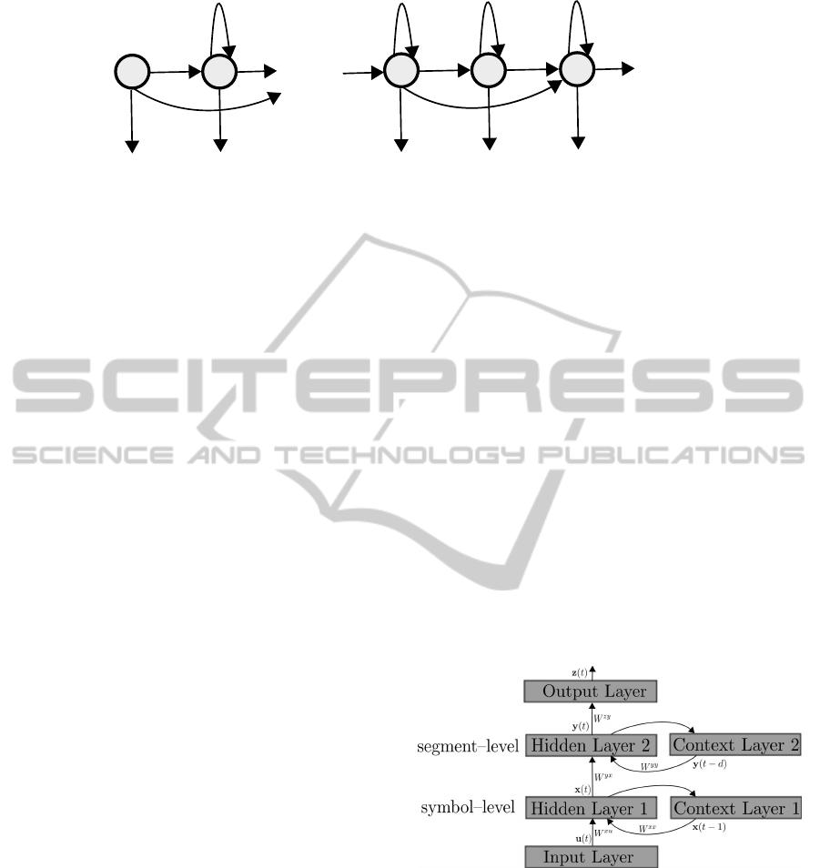
Figure 2 illustrates the SMRNN architecture. It
consists of two simple recurrent networks (SRN) (El-
man, 1990) arranged in an hierarchical fashion. The
first SRN processes the symbol-level and the second
the segment-level of the input sequence. Regarding
the telephone number example, the single digits cor-
respond to symbols processed on symbol-level while
the groups of two/three digits correspond to segments
processed on segment-level.
Figure 2: SMRNN topology.
The SMRNN has an input, output, and two hid-
den layers as it is known from multilayer feedfor-
ward networks. In addition it has two context layers.
These layers have the same number of units as the
corresponding hidden layers and each unit represents
a copy of the last output of the hidden layer. Based
on this topology the network is able to learn temporal
patterns of a sequential input implicitly (Gl¨uge et al.,
2010a; Gl¨uge et al., 2010b).
In the following, we use the receiver-sender-
SEGMENTED-MEMORY RECURRENT NEURAL NETWORKS VERSUS HIDDEN MARKOV MODELS IN
EMOTION RECOGNITION FROM SPEECH
309

notation. The upper index of the weight matrices de-
note the corresponding layer and the lower index the
single units. For example, W
xu
ki
denotes the connec-
tion between the kth unit in hidden layer 1 and the
ith unit in the input layer (cf. Fig. 2). Moreover, f
net
denotes the transfer function of the network (e.g., hy-
perbolic tangent, sigmoid function) and n
u
, n
x
, n
y
, n
z
denote the number of units in the input, hidden 1, hid-
den 2, and output layer.
The introduction of the parameter d on segment-
level makes the main difference between a cascade of
SRNs and an SMRNN. It denotes the length of a seg-
ment, which can be fixed or variable. The processing
of an input sequence starts with the initial symbol-
level state x(0) and segment-level state y(0). At the
beginning of a segment (segment head SH) x(t) is up-
dated with x(0) and input u(t). On other positions
x(t) is obtained from its previous state x(t − 1) and
input u(t). It is calculated by
x
k
(t) =
f
net
∑
n
x
j
W
xx
kj
x
j
(0) +
∑
n
u
i
W
xu
ki
u
i
(t)
,if SH
f
net
∑
n
x
j
W
xx
kj
x
j
(t − 1) +
∑
n
u
i
W
xu
ki
u
i
(t)
,
otherwise
(1)
with k = 1,...,n
x
. The segment-level state y(0) is
updated at the end of each segment (segment tail ST)
as
y
k
(t) =
f
net
∑
n
y
j
W
yy
kj
y
j
(t − 1) +
∑
n
x
i
W
yx
ki
x
i
(t)
,
if ST
y
k
(t − 1), otherwise
(2)
with k = 1, . . . , n
y
. The network output results in for-
warding the segment-level state
z
k
(t) = f
net
n
y
∑
j
W
zy
kj
y
j
(t)
!
with k = 1, . . . ,n
z
.
(3)
The dynamic of an SMRNN is mainly influenced
by the length of the segments d. While the symbol-
level is updated on a symbol by symbol basis, the
segment-level changes only with the end of a seg-
ment, after d symbols are processed. At the end of the
input sequence the segment-levelstate is forwarded to
the output layer to generate the final output. The dy-
namics of an SMRNN processing a sequence is shown
in Fig. 3. In the example the interval d is fixed and the
sequence consists of 3 segments.
For the training of the SMRNN we use an ex-
tention of the real-time recurrent learning algorithm
(eRTRL) as it is described in (Chen and Chaudhari,
2009). During learning the network weights W and
the initial states of the hidden layers x(0), y(0) are
adapted to minimise the sum of squared error at the
output.
3 EXPERIMENTAL SETUP
3.1 Speech Database
We chose the well-known studio recorded Berlin
Emotional Speech Database (EMO-DB) (Burkhardt
et al., 2005) to test the SMRNN approach on emo-
tion recognition from speech. It is freely accessible
and provides high quality audio material and annota-
tion. It is used in several studies on emotion recog-
nition from speech (El Ayadi et al., 2007; Schuller
et al., 2009b; Albornoz et al., 2011). Seven emotional
classes are covered, namely anger, boredom, disgust,
fear, joy, neutral, and sadness.
The corpus consists of ten predefined German sen-
tences that are not emotionally biased by their mean-
ing, e.g., “Der Lappen liegt auf dem Eisschrank” (The
cloth is lying on the fridge). Sentences are spoken
by ten (five male and five female) professional ac-
tors in each emotional way. In a perception test the
recorded utterances were evaluated and deleted when
recognition errors were more than 20% and if they
were judged as non natural by more than 40% of 20
listeners. This ensures the emotional quality and nat-
uralness of the utterances.
For the recognition task each emotional class was
split into 90% training and 10% test data for the
HMMs. Further, the data for the SMRNNs was split
into 80% for training, 10% for validation, and 10%
for testing. The validation set was used to identify
the parameters of the networks (number of neurons in
hidden layers n
x
, n
y
, and length of segments d) that
seem to work best on each class. Afterwards the net-
works were tested on the test data.
Table 1 shows the distribution of the utterances
over the emotion classes.
Table 1: EMO-DB utterances grouped by emotional
class and separation into training/testing or train-
ing/validation/testing.
Emotion No. utterances HMM SMRNN
Anger 127 114/13 102/13/12
Boredom 79 71/8 63/8/8
Disgust 38 34/4 30/4/4
Fear 55 50/5 44/6/5
Joy 64 58/6 51/6/7
Neutral 78 70/8 62/8/8
Sadness 52 47/5 42/5/5
NCTA 2011 - International Conference on Neural Computation Theory and Applications
310
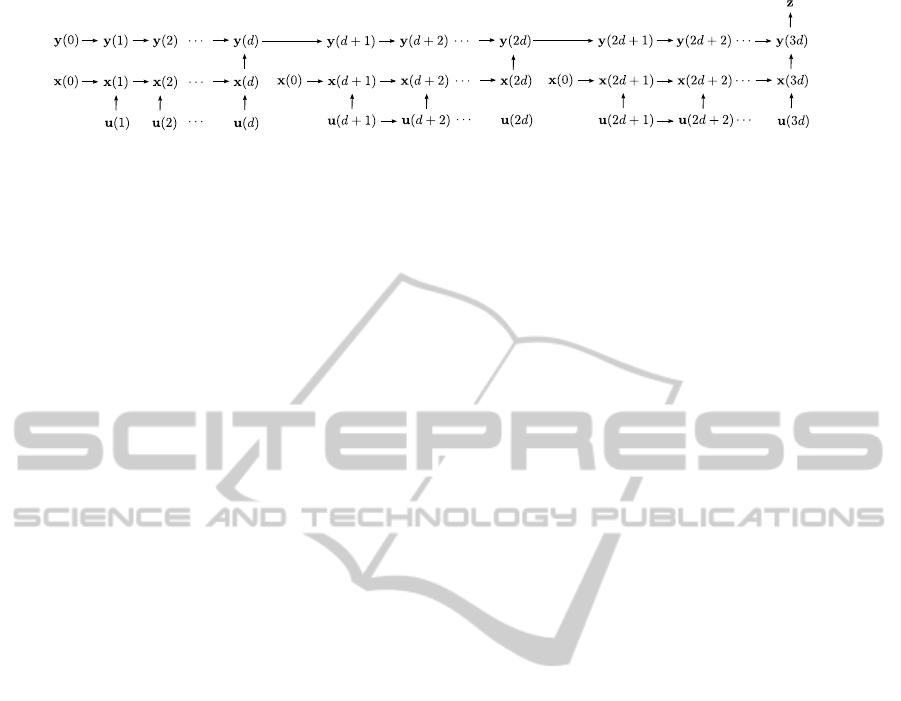
Figure 3: SMRNN dynamics.
3.2 Feature Selection and Extraction
One of the most relevant features for emotion recog-
nition from speech is the pitch . It represents the per-
ceived fundamental frequency (F0) of a sound. Be-
side pitch, spectral features, such as mel-frequency
cepstral coefficients (MFCCs) are dominant features
used for speech recognition. Further, MFCCs are
used in speaker verification (Ganchev et al., 2005)
and even music information retrieval such as genre
classification (M¨uller, 2007). They have also been
found meaningful for emotion recognition (Vlasenko
et al., 2008; Vlasenko and Wendemuth, 2009b; B¨ock
et al., 2010; H¨ubner et al., 2010; Schuller et al., 2011).
MFCCs are coefficients that collectively make up
a mel-frequency cepstrum (MFC). They are derived
from a type of cepstral representation of the audio
clip (a nonlinear “spectrum-of-a-spectrum”). The dif-
ference between the cepstrum and the mel-frequency
cepstrum is that in the MFC, the frequency bands are
equally spaced on the mel scale, which approximates
the human auditory system’s response more closely
than the linearly-spaced frequency bands used in the
normal cepstrum (Fant, 1960).
For our experiment, the features were extracted
with the help of the Hidden Markov Model Toolkit
(Young et al., 2006), primarily used for speech recog-
nition research.
3.2.1 Features for HMMs
The speech data was processed using a 25ms Ham-
ming window, with a frame rate of 10ms. For each
frame (25ms audio material) a 39 dimensional feature
vector was extracted. It consisted of 12 MFCCs and
0th cepstral coefficient plus first and second deriva-
tives, which gives a 39 dimensional feature vector.
The first and second derivatives are so called dy-
namic features that take the temporal variation of the
speech signal into account. In the literature, the first
derivatives are often called Deltas (∆) and the second
derivativesAcceleration (∆∆). This feature set is quite
common in speech community as well as in emotion
recognition from speech.
The mean length of an utterance in EMO-DB is
2.74s. With a frame rate of 10ms this resulted in a
mean of 274 × 39 = 10686 values per utterance.
To compare the results gained by the SMRNNs we
additionaly trained HMMs with a reduced feature set.
Thus, we kept the 12 MFCCs and the 0th coefficient
but generated a set having just the Deltas (26 fea-
tures) and another without any additional derivatives
(13 features).
3.2.2 Features for SMRNNs
For the SMRNNs, we also used a 25ms Hamming
window to process the speech signal. Preliminary
experiments showed that the performance of the net-
works was constant in the range of the frame rate be-
tween 10ms and 25ms. To reduce the computational
effort we chose 25ms for the frame rate, which is the
same size as the Hamming window (no overlapping).
We employed 12 MFCCs and the 0th cepstral co-
efficient, which gives a 13 dimensional feature vector.
Note that we did not use the dynamic features (first
and second derivatives) as the network should learn
the temporal structure of the data. Due to the sig-
moidal characteristics of the activation function used
in the networks the features were scaled onto values
in the range of [−7,7].
With the mean length of an utterance of 2.74s and
the frame rate of 25ms we got 110× 13= 1430 values
per utterance. The larger frame rate and the reduction
of the features led to around 7.5 times less data than
it was used for the HMM approach.
3.3 Architecture of the Classifier
Both types of classifiers work according to the one-
class-one-classifier principle. We employ seven clas-
sifiers and each is trained on one emotional class. In
the end the output of these seven ‘experts’ is used to
find the final decision. Figure 4 illustrates the ap-
proach.
3.3.1 HMM
In case of Hidden Markov Models for each class one
model was trained. In testing, the input was presented
to each model simultaneously and by traversing the
model the most likely path through it was computed
using the Viterbi-Algorithm. Finally, for each result
the log-likelihood was calculated. According to these
SEGMENTED-MEMORY RECURRENT NEURAL NETWORKS VERSUS HIDDEN MARKOV MODELS IN
EMOTION RECOGNITION FROM SPEECH
311
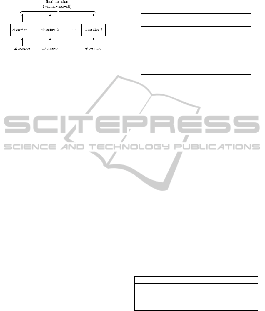
Figure 4: One-class-one-classifier principle.
values a final decision was carried out, i.e., the largest
value was taken, which is a winner-take-all principle.
The training and testing was done by utilising the Hid-
den Markov Toolkit (Young et al., 2006) by the Uni-
versity of Cambridge.
In particular, an HMM had the following struc-
ture: It was a left-to-right forward passing scheme,
which means that all connections were either forward
oriented or self-loops (cf. Fig. 1). Moreover, each
model had 3 internal states that is standard in speech
processing. The input was the sequence of feature
vectors of an utterance and the output produced by
the system was the emotion label (cf. Sec. 3.1).
3.3.2 SMRNN
According to the general structure of the classifier (cf.
Fig. 4) we trained seven different SMRNNs. Each
consists of thirteen input units (n
u
= 13) and one out-
put unit (n
z
= 1), such that each network decided
whether the presented utterance belongs to its class
(z = 1) or not (z = 0). The transfer function for
the hidden and output units was the sigmoid function
( f
net
(x) = 1/(1+ exp(−x)) ). The input units simply
forwarded the input data. Initial weights were set to
uniformly distributed random values in the range of
[−0.4, 0.4].
Each network differs in three parameters, namely
the number of units in the hidden layers n
x
, n
y
, and
the length of the segments d. They were determined
using the training and validation set. Those param-
eter combinations that worked best on the validation
set after training were picked for the final classifier.
Due to the computational effort for network training
we used no systematic search technique for combina-
tions of parameters yet. In this respect, the present
parameter combinations should be taken as an edu-
cated guess. Table 2 shows the network configuration
for each class.
The networks were trained for 100 epochs with
the learning rate 0.2 and momentum 0.1. For each
utterance the networks delivered an output value in
the range of (0, 1). To come up with a final deci-
sion, we used the winner-take-all principle, that is, the
Table 2: SMRNN configuration grouped by emotional
class.
Emotion hidden 1 hidden 2 segment
n
x
n
y
length d
Anger 28 8 17
Boredom 19 8 14
Disgust 22 14 8
Fear 17 17 7
Joy 19 29 2
Neutral 8 26 19
Sadness 13 13 11
network with the highest output determined the emo-
tional class that corresponds to the utterance.
4 RESULTS
The performance of both classification methods was
measured using the weighted average (WA) of class-
wise accuracy as it is proposed in (Schuller et al.,
2009a). Since the number of utterances in the single
classes differed considerably, the weighted average
provides a more reasonable measure than the arith-
metic mean (unweighted average UA).
In the following, HMM denotes the classifier that
was trained using the 13 basic features (12 MFCCs
plus 0th coefficient). HMM∆ denotes the classifier
that was trained with 26 features (13 basic features
plus first derivatives). HMM∆∆ denotes the HMM
classifier that was trained with the full set of 39 fea-
tures (13 basic features plus first and second deriva-
tives).
Table 3 shows the results for the SMRNN against
the HMM approach using the weighted and un-
weighted average.
Table 3: Weighted and unweighted average of class-wise
accuracy in % for HMM and SMRNN classifiers during
training and testing.
Emotion training WA / UA testing WA / UA
SMRNN 91.08 / 91.62 71.02 / 73.47
HMM∆∆ 79.70 / 81.76 73.75 / 77.55
HMM∆ 81.17 / 81.08 60.03 / 63.27
HMM 71.15 / 70.72 51.72 / 55.10
The SMRNN classifier performed best during
training (≈ 91%), but dropped down to 71% in test-
ing. HMM∆∆ delivered the best result on the test set
(≈ 74%). This coincides with the results reported in
(Schuller et al., 2009b) and (B¨ock et al., 2010).
Feature reduction caused a significant decrease in
the performance of the HMMs. The HMM∆ and
NCTA 2011 - International Conference on Neural Computation Theory and Applications
312

HMM classifiers (cf. Tab. 3) performed inferior to the
SMRNNs.
In comparison to the HMM∆∆ the SMRNNs per-
formed slightly worse (71.02% vs. 73.75% on test
set). Note that the networks used three times less fea-
tures (13 vs. 39, cf. Sec. 3.2.2) than the HMM∆∆ and
reached a comparable performance.
Tables 4 and 5 show the class-wise accuracy of the
SMRNN and HMM∆∆ classifier.
Table 4: Confusion matrix of SMRNN classifier on test set
with class-wise accuracy in % (Acc.).
Emotion A B D F J N S
Anger 12 0 0 1 2 0 1
Boredom 0 5 0 0 0 3 0
Disgust 0 0 3 0 0 0 0
Fear 0 0 0 3 1 0 0
Joy 0 0 1 0 4 0 0
Neutral 0 1 0 1 0 5 0
Sadness 0 2 0 0 0 0 4
Acc. 100 62.5 75 60 57 62.5 80
Table 5: Confusion matrix of HMM∆∆ classifier on test set
with class-wise accuracy in % (Acc.).
Emotion A B D F J N S
Anger 11 0 0 1 2 0 0
Boredom 0 7 0 1 0 1 1
Disgust 0 0 2 0 0 0 0
Fear 1 0 0 3 0 0 0
Joy 1 0 0 0 4 0 0
Neutral 0 0 0 0 0 7 0
Sadness 0 1 2 0 0 0 4
Acc. 84.6 87.5 50 60 66.7 87.5 80
One can see that for SMRNNs as for HMM∆∆
the accuracy on the different classes was nonhomoge-
neous. Both classifiers performed well on anger and
sadness (Acc. ≥ 80%) but performed worse on fear
and joy (Acc. < 70%). Anger was perfectly classified
by the SMRNNs. This might be due to the overrepre-
sentation of anger in the database (cf. Tab. 1). Further,
some emotions (e.g., disgust and sadness) occure in a
small number in the test set. Therefore, the correct
classification of one of the utterances in that classes
had a high impact on the overall performance.
5 DISCUSSION
Our experiment showed that SMRNNs have the po-
tential to solve complex sequence classification tasks
as they appear in automatic speech processing. The
memory for contextual information enables the net-
work to learn long-term as well as short-term tempo-
ral dependencies, while the segmentation of the mem-
ory prevents it to suffer from the vanishing gradient
problem. As the networks are able to learn the dy-
namics of the input sequences it is not necessary to
provide the dynamic features of the speech signal to
learn the task.
In the experiment SMRNNs performed slightly
worse (≈ 3% on test set) compared to HMMs
that were trained with three times more features
(HMM∆∆). Further, the input signal of the HMMs
was sampled more frequently during feature extrac-
tion (10ms for HMMs vs. 25ms for SMRNNs, cf. Sec.
3.2.2). In total the HMM∆∆s were trained with 7.5
times more data than the SMRNNs.
On the other hand, HMMs that used the same
amount of features were outperformed by the SM-
RNNs by around 19% weighted average accuracy on
the test set (cf. Tab. 3).
The perfect classification of anger by the SM-
RNNs (cf. Tab. 4) gives rise to the hope, that the per-
formance of the networks could enhance by providing
more training material for the different classes.
We see the main drawback of the SMRNN ap-
proach in the computational costs for the network
training. In worst-case (network is fully connected
and all weights are adaptable) the RTRL algorithm
has a space complexity Θ(n
3
) and average time com-
plexity Θ(n
4
), with n denoting the number of units in
the network (Williams and Zipser, 1995). By now,
this forced us to guess the parameter combinations
(n
x
,n
y
,d) for the networks. The learning rate, mo-
mentum and number of epochs for the training might
also not be optimal yet. Replacement of the RTRL
algorithm by the extended Kalman filter algorithm
(EKF) could be a possible solution for the problem
(
ˇ
Cerˇnansk´y and Beˇnuˇskova, 2003).
Beside the optimisation of the network parameter,
there are indications that the networks performance
can be improved with the use of alternative features,
e.g., perceptual linear prediction coefficients (Her-
mansky, 1990).
ACKNOWLEDGEMENTS
The authors acknowledge the support provided
by the federal state Sachsen-Anhalt with the
Graduiertenf¨orderung (LGFG scholarship). Fur-
thermore, we acknowledge continued support by
the Transregional Collaborative Research Centre
SFB/TRR 62 “Companion-Technology for Cognitive
Technical Systems” funded by the German Research
SEGMENTED-MEMORY RECURRENT NEURAL NETWORKS VERSUS HIDDEN MARKOV MODELS IN
EMOTION RECOGNITION FROM SPEECH
313

Foundation (DFG). We also acknowledge the DFG
for financing our computing cluster used for parts of
this work.
REFERENCES
Albornoz, E. M., Milone, D. H., and Rufiner, H. L. (2011).
Spoken emotion recognition using hierarchical clas-
sifiers. Computer Speech and Language, 25(3):556–
570.
Baum, L., Petrie, T., Soules, G., and Weiss, N. (1970).
A maximization technique occurring in the statistical
analysis of probabilistic functions of markov chains.
Ann. Math. Stat., 41:164–171.
Bengio, Y., Simard, P., and Frasconi, P. (1994). Learning
long-term dependencies with gradient descent is diffi-
cult. IEEE transactions on neural networks, 5(2):157–
66.
B¨ock, R., H¨ubner, D., and Wendemuth, A. (2010). De-
termining optimal signal features and parameters for
hmm-based emotion classification. In MELECON
2010 - 15th IEEE Mediterranean Electrotechnical
Conference, pages 1586–1590.
Boreczky, J. S. and Wilcox, L. D. (1998). Hidden markov
model framework for video segmentation using audio
and image features. In ICASSP, IEEE International
Conference on Acoustics, Speech and Signal Process-
ing, volume 6, pages 3741–3744.
Burkhardt, F., Paeschke, A., Rolfes, M., Sendlmeier, W.,
and Weiss, B. (2005). A database of german emo-
tional speech. In Proceedings of the 9th European
Conference on Speech Communication and Technol-
ogy; Lisbon, pages 1517–1520.
Chen, J. and Chaudhari, N. (2009). Segmented-memory
recurrent neural networks. Neural Networks, IEEE
Transactions, 20(8):1267–80.
Ekman, P. (July 1992). Are there basic emotions? Psycho-
logical Review, 99:550–553.
El Ayadi, M., Kamel, M., and Karray, F. (2007). Speech
emotion recognition using gaussian mixture vector au-
toregressive models. In Acoustics, Speech and Signal
Processing, 2007. ICASSP 2007. IEEE International
Conference on, volume 4, pages 957–960. IEEE.
El Ayadi, M., Kamel, M. S., and Karray, F. (2011). Sur-
vey on speech emotion recognition: Features, classi-
fication schemes, and databases. Pattern Recognition,
44(3):572–587.
Elman, J. L. (1990). Finding structure in time. Cognitive
Science, 14(2):179–211.
Fant, G. (1960). Acoustic theory of speech production.
Mounton, The Hague.
Ganchev, T., Fakotakis, N., and Kokkinakis, G. (2005).
Comparative evaluation of various mfcc implementa-
tions on the speaker verification task. In Proc. of the
SPECOM, pages 191–194.
Gl¨uge, S., B¨ock, R., and Wendemuth, A. (2010a). Im-
plicit sequence learning - a case study with a 4-2-4
encoder simple recurrent network. In Proceedings of
the International Conference on Fuzzy Computation
and 2nd International Conference on Neural Compu-
tation, pages 279–288.
Gl¨uge, S., Hamid, O. H., and Wendemuth, A. (2010b). A
simple recurrent network for implicit learning of tem-
poral sequences. Cognitive Computation, 2(4):265–
271.
Grimm, M., Kroschel, K., Mower, E., and Narayanan, S.
(2007). Primitives-based evaluation and estimation of
emotions in speech. Speech Communication, 49(10-
11):787–800.
Hermansky, H. (1990). Perceptual linear predictive (PLP)
analysis of speech. Journal of the Acoustical Society
of America, 87(4):1738–1752.
Hitch, G. J., Burgess, N., Towse, J. N., and Culpin, V.
(1996). Temporal grouping effects in immediate re-
call: A working memory analysis. Quarterly Journal
of Experimental Psychology Section A: Human Exper-
imental Psychology, 49(1):116–139.
Hochreiter, S. (1998). The vanishing gradient problem dur-
ing learning recurrent neural nets and problem solu-
tions. International Journal of Uncertainty, Fuzziness
and Knowledge-Based Systems, 6(2):107–116.
H¨ubner, D., Vlasenko, B., Grosser, T., and Wendemuth,
A. (2010). Determining optimal features for emo-
tion recognition from speech by applying an evolu-
tionary algorithm. In INTERSPEECH 2010, pages
2358–2361.
Inoue, T., Nakagawa, R., Kondou, M., Koga, T., and Shi-
nohara, K. (2011). Discrimination between mothers’
infant- and adult-directed speech using hidden markov
models. Neuroscience Research, 70(1):62–70.
Kim, W. and Hansen, J. (2010). Angry emotion detec-
tion from real-life conversational speech by leverag-
ing content structure. In Acoustics Speech and Signal
Processing (ICASSP), 2010 IEEE International Con-
ference on, pages 5166–5169.
Mehrabian, A. (1996). Pleasure-arousal-dominance: A gen-
eral framework for describing and measuring individ-
ual differences in temperament. Current Psychology,
14(4):261–292.
M¨uller, M. (2007). Information Retrieval for Music and
Motion. Springer Verlag.
Nicholson, J., Takahashi, K., and Nakatsu, R. (1999). Emo-
tion recognition in speech using neural networks. In
Neural Information Processing, 1999. Proceedings.
ICONIP ’99. 6th International Conference on, vol-
ume 2, pages 495–501.
Nwe, T. L., Foo, S. W., and Silva, L. C. D. (2003). Speech
emotion recognition using hidden markov models.
Speech Communication, 41(4):603–623.
Petrushin, V. A. (2000). Emotion recognition in speech
signal: experimental study, development, and appli-
cation. In Proceedings of the ICSLP 2000, volume 2,
pages 222–225.
Pierre-Yves, O. (2003). The production and recognition of
emotions in speech: features and algorithms. Inter-
national Journal of Human-Computer Studies, 59(1-
2):157 – 183. Applications of Affective Computing in
Human-Computer Interaction.
Rabiner, L. and Juang, B.-H. (1993). Fundamentals of
NCTA 2011 - International Conference on Neural Computation Theory and Applications
314

Speech Recognition. Prentice Hall, New Jersey, 8th
edition.
Scherer, S., Oubbati, M., Schwenker, F., and Palm, G.
(2008). Real-time emotion recognition using echo
state networks. In Andr´e, E., Dybkjr, L., Minker, W.,
Neumann, H., Pieraccini, R., and Weber, M., editors,
Perception in Multimodal Dialogue Systems, volume
5078 of Lecture Notes in Computer Science, pages
200–204. Springer Berlin / Heidelberg.
Schmidt, M., Schels, M., and Schwenker, F. (2010). A
hidden markov model based approach for facial ex-
pression recognition in image sequences. In Lecture
Notes in Computer Science (including subseries Lec-
ture Notes in Artificial Intelligence and Lecture Notes
in Bioinformatics), volume 5998 LNAI, pages 149–
160. Springer.
Schuller, B., Batliner, A., Steidl, S., and Seppi, D. (2011).
Recognising realistic emotions and affect in speech:
State of the art and lessons learnt from the first chal-
lenge. Speech Communication. Article in Press.
Schuller, B., Rigoll, G., and Lang, M. (2004). Speech
emotion recognition combining acoustic features and
linguistic information in a hybrid support vector
machine-belief network architecture. In Acoustics,
Speech, and Signal Processing, 2004. Proceedings.
(ICASSP ’04). IEEE International Conference on, vol-
ume 1, pages I – 577–80 vol.1.
Schuller, B., Steidl, S., and Batliner, A. (2009a). The in-
terspeech 2009 emotion challenge. In Tenth Annual
Conference of the International Speech Communica-
tion Association, pages 312–315.
Schuller, B., Vlasenko, B., Eyben, F., Rigoll, G., and
Wendemuth, A. (2009b). Acoustic emotion recog-
nition: A benchmark comparison of performances.
In Automatic Speech Recognition & Understanding,
2009. ASRU 2009. IEEE Workshop on, pages 552–
557. IEEE.
Severin, F. T. and Rigby, M. K. (1963). Influence of digit
grouping on memory for telephone numbers. Journal
of Applied Psychology, 47(2):117–119.
Song, M., You, M., Li, N., and Chen, C. (2008). A robust
multimodal approach for emotion recognition. Neuro-
computing, 71(10-12):1913–1920.
Trentin, E., Scherer, S., and Schwenker, F. (2010). Max-
imum echo-state-likelihood networks for emotion
recognition. In Schwenker, F. and El Gayar, N., ed-
itors, Artificial Neural Networks in Pattern Recogni-
tion, volume 5998 of Lecture Notes in Computer Sci-
ence, pages 60–71. Springer Berlin / Heidelberg.
Tuzlukov, V. P. (2000). Signal Detection Theory.
Birkh¨auser, Boston.
ˇ
Cerˇnansk´y, M. and Beˇnuˇskova, L. (2003). Simple recur-
rent network trained by rtrl and extended kalman filter
algorithms. Neural Network World, 13(3):223–234.
Ververidis, D. and Kotropoulos, C. (2006). Emotional
speech recognition: Resources, features, and methods.
Speech Communication, 48(9):1162–1181.
Viterbi, A. J. (1967). Error bounds for convolutional codes
and an asymptotically optimal decoding algorithm.
IEEE Transactions on Information Theory, 13:260–
269.
Vlasenko, B., Schuller, B., Wendemuth, A., and Rigoll, G.
(2008). On the influence of phonetic content vari-
ation for acoustic emotion recognition. In Percep-
tion in Multimodal Dialogue Systems, volume 5078 of
Lecture Notes in Computer Science, pages 217–220.
Springer Berlin / Heidelberg.
Vlasenko, B. and Wendemuth, A. (2009a). Heading toward
to the natural way of human-machine interaction: the
nimitek project. In Multimedia and Expo, 2009. ICME
2009. IEEE International Conference on, pages 950–
953.
Vlasenko, B. and Wendemuth, A. (2009b). Processing af-
fected speech within human machine interaction. In
INTERSPEECH-2009, volume 3, pages 2039–2042,
Brighton.
Williams, R. J. and Zipser, D. (1995). Gradient-based
learning algorithms for recurrent networks and their
computational complexity, pages 433–486. L. Erl-
baum Associates Inc., Hillsdale, NJ, USA.
W¨ollmer, M., Eyben, F., Reiter, S., Schuller, B., Cox, C.,
Douglas-Cowie, E., and Cowie, R. (2008). Aban-
doning emotion classes - towards continuous emotion
recognition with modelling of long-range dependen-
cies. In INTERSPEECH-2008, pages 597–600.
Yingthawornsuk, T. and Shiavi, R. (2008). Distinguishing
depression and suicidal risk in men using gmm based
frequency contents ofaffective vocal tract response. In
Control, Automation and Systems, 2008. ICCAS 2008.
International Conference on, pages 901–904.
Young, S. J., Evermann, G., Gales, M. J. F., Hain, T., Ker-
shaw, D., Moore, G., Odell, J., Ollason, D., Povey, D.,
Valtchev, V., and Woodland, P. C. (2006). The HTK
Book, version 3.4. Cambridge University Engineering
Department, Cambridge, UK.
SEGMENTED-MEMORY RECURRENT NEURAL NETWORKS VERSUS HIDDEN MARKOV MODELS IN
EMOTION RECOGNITION FROM SPEECH
315
