KINETIC MORPHOGENESIS OF A MULTILAYER PERCEPTRON

Bruno Apolloni

, Simone Bassis

and Lorenzo Valerio

Department of Computer Science, University of Milan, via Comelico 39/41, 20135 Milan, Italy

Department of Mathematics “Federigo Enriques”, University of Milan, via Saldini 50, 20133 Milan, Italy

Keywords:

Neural network morphogenesis, Mobile neurons, Deep multilayer perceptrons, Eulerian dynamics.

Abstract:

We introduce a morphogenesis paradigm for a neural network where neurons are allowed to move au-

tonomously in a topological space to reach suitable reciprocal positions under an informative perspective.

To this end, a neuron is attracted by the mates which are most informative and repelled by those which are

most similar to it. We manage the neuron motion with a Newtonian dynamics in a subspace of a framework

where topological coordinates match with those reckoning the neuron connection weights. As a result, we

have a synergistic plasticity of the network which is ruled by an extended Lagrangian where physics com-

ponents merge with the common error terms. With the focus on a multilayer perceptron, this plasticity is

operated by an extension of the standard back-propagation algorithm which proves robust even in the case of

deep architectures. We use two classic benchmarks to gain some insights on the morphology and plasticity we

are proposing.

1 INTRODUCTION

A couple of factors determining the success of com-

plex biological neural networks, such as our brain,

is represented by a suited mobility of neurons during

the embrional stage along with a selective formation

of synaptic connections out of growing axons (Mar´ın

and Lopez-Bendito, 2007). While the second aspect

has been variously considered in artiﬁcial neural net-

works, for instance in the ART algorithms (Carpenter

and Grossberg, 2003), the morphogenesis of artiﬁcial

neural networks has been mainly intended as the out-

put of evolutionary algorithms which are deputed to

identify its most convenient layout (Stanley and Mi-

ikkulainen, 2002). Rather, in this paper we focus on a

true mobility of the neurons in the topological space

where they are located.

To bypass the complexity of the chemical and

electrochemical phenomena at the basis of the brain

morphology (Mar´ın and Rubenstein, 2003), we prefer

to rule the artiﬁcial neuron motion through a classical

Newtonian dynamics which is governed by clean and

simple laws. On the one hand, we look for an efﬁcient

assessment of the location of the neurons which pro-

motes the specialization of their computational task

as a part of the overall functionality of the neural net-

work they belong to. In this sense, we borrow from

the old trade unions’ slogan “work less, work all” the

aim of a fair distribution of cognitive and computa-

tional loads on each neuron. On the other hand, w.r.t.

a multilayer perceptron (MLP) architecture, we assign

the concrete realization of this aim to two antagonist

forces within a potential ﬁeld: i) an attraction force

from the upward layer neurons to the downward layer

ones, which is determined by the masses of any pair

of mates, which in turn we identify with the delta term

of the back-propagation algorithm; and ii) a repul-

sive force between similar neurons in the same layer,

where similarity is appreciated in terms of their vec-

tors of outgoing connection weights. The potentials

associated to these forces plus the induced kinemat-

ics concur on the deﬁnition of the Hamiltonian of the

motion (Feynman et al., 1963), which we integrate

with other energetic terms coming from the cognitive

goals of the network: namely, a quadratic error term

plus an entropic term in the realm of feature extrac-

tion algorithms. This extended Hamiltonian consti-

tutes the cost function of a standard back-propagation

algorithm which synergistically adapts weights and

locations of the single neurons.

We check the beneﬁts of this contrivanceon a cou-

ple of demanding benchmarks available on the web.

Actually, we do not claim that our training proce-

dure outperforms the best algorithms in the literature.

Rather, we realize the robustness of our results within

a reviving paradigm of a general-purpose learner with

a very essential training strategy. The core of our ex-

perimental analysis is a preliminary characterization

Apolloni B., Bassis S. and Valerio L..

KINETIC MORPHOGENESIS OF A MULTILAYER PERCEPTRON.

DOI: 10.5220/0003642800990105

In Proceedings of the International Conference on Neural Computation Theory and Applications (NCTA-2011), pages 99-105

ISBN: 978-989-8425-84-3

 2011 SCITEPRESS (Science and Technology Publications, Lda.)

of the morphogenesis functionality which enriches

the complexity of the training behavior without lead-

ing to chaotic or diverging trends.

The paper is organized as follows. In Section 2

we describe the dynamics of the neurons. Then we

resume the main features of the related learning pro-

cedure in Section 3. We toss the procedure on bench-

marks in Section 4. In the ﬁnal section we draw some

conclusions and outline future work.

2 A DYNAMICS OF THE

NEURONS

Let us consider an r-layer MLP where all neurons of

a layer are located in a Euclidean (two-dimensional,

by default) space X. Moreover let us ﬁx the layout

notation, where subscript j refers to neurons lying on

layer ℓ + 1, i, i

′

to those located in layer ℓ, and ℓ runs

through the r layers. We rule the activation of the

generic neuron by:

= f(net

); net

ℓ

∑

i=1

; λ

= e

−µd

(1)

where τ

is the state of the j-th neuron, w

the weight

of the connection from the i-th neuron (with an addi-

tional dummy connection in the role of neuron thresh-

old), ν

ℓ

the number of neurons lying on layer ℓ, and

f the activation function. In addition λ

is a penalty

factor depending on the topological distance d

be-

tween the two neurons. Namely, d

= k x

− x

where x

denotes the position of the neuron within its

layer. This factor affects the net-input net

of the j-th

neuron in an unprecedented way by linking the infor-

mation piped through the network to the dynamics of

the neurons. Thus, we complete the description of the

network by specifying the potential ﬁeld where the

neurons, in the role of particles, are embedded.

With reference to Figure 1, generated by the neu-

rons of two contiguous layers (ℓ, ℓ + 1), on each neu-

ron i of layer ℓ we have a couple of forces (A,R):

A = G

; R = k

′

(l − d

′

)

(2)

where (x)

= max{0, x}, representing a gravitational

force between the masses m

with inter-layer dis-

tance ζ

, and a repulsive force between neurons i, i

′

at intra-layer distance d

′

, respectively. As for the for-

mer, we assume ζ

to be a large constant h resuming

the square root of G as well. We may ﬁgure the lay-

ers lying on parallel planes which are very far each

With k · k

we denote the L

-norm, where i = 2 is as-

sumed wherever not expressly indicated in the subscript.

Figure 1: Potential ﬁeld generated by both attractiveupward

neurons (black bullets) and repulsive siblings (gray bullets).

The bullet size is proportional to the strength of the ﬁeld,

hence either to the neuron mass (black neurons) or to the

outgoing connection weight averaged similarity (gray neu-

rons). Arrows: stream of the potential ﬁeld; black contour

lines: isopotential curves.

other; in this respect d

in (1) represents the length

of projection of the vector from the i-th to the j-th

neuron on the downward layer. The right hand side

term in (2) is an l-repulsive force which is 0 if d

′

> l.

To conclude the model, we identify the mass of the

neurons with their information content which in our

back-propagationtraining procedure is represented by

the back-piped error term δ (see Section 3). After nor-

malizing in order to maintain constant the total mass

on each layer, its expression reads: m

|δ

kδk

. More-

over, the elastic constant k

′

hinges on how similar the

normed weight vectors are, i.e. on the modulus of the

cosine of the angle between them:

′



· w

′

k · kw

′



(3)

The dynamics of this system is ruled by the Hamilto-

nian:

H = ξ

+ ξ

(4)

for suitable ξ

s, with

∑

i, j

; P

∑

i,i

′

(l − d

′

)

;

∑

(5)

where the latter is connected to the kinetic energy in

correspondence of the neuron velocities v

s. The mo-

tion driven by this Hamiltonian is ruled by the accel-

eration:

NCTA 2011 - International Conference on Neural Computation Theory and Applications

100

= ξ

∑

sign(x

− x

)−

∑

′

(l − d

′

)

sign(x

′

− x

) (6)

for proper ξ

s. Actually, for simplicity’s sake we em-

bed the mass of the accelerated particle into ξ

. Since

this mass is not a constant, it turns out to be an abuse

which makes us forget some sensitivity terms during

the training of the network. Moreover, in order to

guide the system toward a stable conﬁguration, we

add a viscosity term which is inversely proportional

to the actual velocity, namely −ξ

. However we

do not reckon the potential linked to this term within

the Lagrangian addends for analogous simplicity rea-

sons. During the training of the MLP, we consider the

following companion potentials driving the neurons

in the coordinate space reporting the weights of their

outgoing connections, according to (LeCun, 1988):

1. an error function that we identify with the custom-

ary quadratic error on the output layer, hence:

∑

(τ

− z

)

(7)

with z

target of the network at the o-th output

neuron, and

2. an entropic term devoted to promoting a represen-

tation of the neuron state vector through Boolean

Independent Components (Apolloni et al., 2009)

via the Schur-concave function (Kreutz-Delgado

and Rao, 1998) – the BICA term:

= ln

∏

−τ

(1− τ

)

−(1−τ

)

(8)

for the state vector τ lying in the Boolean hyper-

cube (for instance computed by a sigmoidal acti-

vation function).

As a conclusion, we ﬁgure the neuron motion within

the whole coordinate space to be ruled by the ex-

tended Hamiltonian L constituted by the sum of both

physical and cognitive terms:

H = ξ

+ ξ

(9)

where the links between the two half-spaces are tuned

by: i) the λ

coefﬁcients in the computation of the

net-input, and ii) the cognitive masses m

of the neu-

rons.

3 TRAINING THE NETWORK

In our framework morphogenesis is the follow-out

of learning. The functional solution of the Hamilto-

nian equations deriving from (9) leads to a Newtonian

dynamics in an extended potential ﬁeld. Rather, its

parametric minimization identiﬁes the system ground

state which according to quantum mechanics denotes

the most stable of the system equilibrium conﬁgura-

tions (Dirac, 1982). Actually, the framing of neural

networks into the quantum physics scenario has been

variously challenged in recent years (Ezhov and Ven-

tura, 2000). However these efforts mainly concern the

quantum computing ﬁeld, hence enhanced computing

capabilities of the neurons. Here we consider conven-

tional computations and classical mechanics. Rather,

superposition aspects concern the various endpoints

of learning trajectories. Many of them may prove in-

teresting (say, stretching valuable intuitions). But a

few, possibly one, attain stability with a near to zero

entropy – a condition which we strengthen through

the additional viscosity term. In turn, we use back-

propagation as an effective minimization method to

move toward the ground state and reread the entire

goal in terms of a MLP training problem.

In comparison to the many new strategies consid-

ered to cope with difﬁcult learning problems, such

as kernel methods (Danafar et al., 2010), restricted

Boltzmann machines (Hinton et al., 2006) and so

on, we assume that most of the goals they pursue

are implicitly resumed by the components of our ex-

tended Hamiltonian in terms of: i) emerging struc-

tures among data, ii) feature selection, iii) group-

ing of specialized branches of the network, and iv)

wise shaking of their state to be unstuck from local

minima. The technicalities of implementing back-

propagation in our framework concern simply an ac-

curate reckoning of the derivatives of the cost func-

tion along the layers. The excerpt of this is reported

in Table 1.

Summing up, we run the two (forward and back-

ward) phases of the training procedure as usual. But

we must be particularly careful about updating not

only the state vector, but also the positions of the neu-

rons during the forward phase on the basis of the ac-

celerations determined by the potential ﬁeld.

4 NUMERICAL EXPERIMENTS

We are left with both a synergistic physics-cognitive

contrivance to move neurons in an MLP and a bet

that this motion helps learning even in the most

highly demanding instances of deep neural net-

works (Larochelle et al., 2009). So what we get is

not a mere layout shaking but a truly efﬁcient neural

network morphogenesis.

To check this functionality, we train two 5-layer

MLPs as in Figures 2(a) and (c) on two benchmarks

KINETIC MORPHOGENESIS OF A MULTILAYER PERCEPTRON

101

Table 1: Gradient expressions for the backward phase from the second to the last layer down.

err.

∂(E

+ E

)

∂w



1−

− x

)

∂x

∂w



;

(10)

= f

′

(net

)

−γln



1− τ



∑

k j

; γ =

pot.

∂P

∂w

= m

sign(δ

)

kδk

(1− m

) f

′

(net

)δ

(11)

∂P

∂w

∑

′

(l − d

′

)

∂k

′

∂w

′

(l − d

′

)

′

− x

)

∂x

∂w

(12)

∂P

∂w

sign(δ

)

kδk

(1− m

) f

′

(net

)δ

+ m

∂v

∂w

(13)

dyn.

∂a

(n)

∂w

= −ξ



∑

′

((l − d

′

)

)sign(x

′

− x

)

∂k

′

∂w

−

∑

′

sign(x

′

− x

)

∂d

′

∂w



(14)

∂k

′

∂w

= sign



· w

′

k · kw

′



′

k · kw

′

k − hw

· w

′

(kw

k · kw

′

(15)

that are representative of a regression and a classiﬁca-

tion demanding task, respectively. They are:

1. The Pumadyn benchmark pumadyn8-nm (Corke,

1996). It consists of 8,192 samples, each consti-

tuted by 8 inputs and one output which are related

by a complex nonlinear equation plus a moderate

noise, which we process through a 8×100×80×

36×1 architecture. Neurons are distributed on the

crosses of a square grid centered in (0,0) in each

layer, with a 100 long edge.

2. The MNIST benchmark (LeCun et al., 1998). It

consists of a training and a test set of 60, 000 and

10,000 examples, respectively, of handwritten in-

stances of the ten digits. Each example contains a

28×28 grid of 256-valued gray shades. We pro-

cess it with a 196× 120×80×36×10 architecture,

where: i) the input neurons are reduced by

w.r.t. the image pixels by simply mediating con-

tiguous pixels, ii) the 10 output neurons lie over

a circle of ray 50, thus referring to a unary rep-

resentation where a single neuron is assigned to

answer 1 and the others 0 on each digit, and iii)

the neurons of the remaining layers are on a grid

as above.

Without exceedingly stressing the network capabili-

ties (we rely on around 20,000 weight updates with

a batch size equal to 20, and a moderate effort to

tune the parameters per each benchmark), we drive

the training process toward local minima in a good

position, though not the best, when compared to the

results available in the literature.

Namely, as for the regression task, we get the

mean squared errors (MSEs) in Table 2 within the

Delve testing framework (Rasmussen et al., 1996).

They locate our method in an intermediate position

Table 2: Regression performances on pumadyn8-nm for dif-

ferent training set sizes.

tr. set size 64 128 256 512 1024

MSE

mean

5.255 2.245 1.818 1.283 1.213

std. (0.541) (0.154) (0.957) (0.036) (0.034)

w.r.t. typical competitors, losing out against sophis-

ticated algorithms that rely either on special imple-

mentations of back-propagation (such as those bas-

ing on ensembles or validation sets) or on other train-

ing rationale (such as kernel SVM (Danafar et al.,

2010)). In turn the addition of both BICA term and

neuron mobility constitutes a real beneﬁt in respect

to the standard back-propagation. We highlight the

learning improvement in Figure 3 where we train the

same network by exploiting these different facilities.

In any case, the graphs denote both a stable behavior

of the training algorithm and unbiased shifts between

desired and computed outputs.

Analogously, the confusion matrix in Table 3 de-

scribes the performances in MNIST classiﬁcation,

while the course of the test error on the single digits

is reported in Figure 4.

We get an error rate equal to 3.2%, that is poorer

when compared to the best performances on this task

which attest at around one order less (Ciresan et al.,

2010). Nevertheless we are able to classify digits

which would prove ambiguous even to a human eye in

spite of the rough compression of the input (see Fig-

ure 5). Moreover, the MSE descent of the ten digits

in Figure 4 denotes a residual training capability that

could be achieved in a longer training session. We re-

mark that, to train the network, we use a batch size of

20 examples randomly drawn from the 60,000 long

training set, whereas the error reported in Figure 4 is

measured on 200 new examples. Thus the curves con-

NCTA 2011 - International Conference on Neural Computation Theory and Applications

102

- 50

(a)

- 20

(b)

- 50

(c)

100

(d)

Figure 2: Initial (a) and ﬁnal (b) network layouts for Pumadyn dataset. Initial layout (c) and 2-nd, 3-rd (left and right half

section resp.) layer neuron trajectories from starting (gray bullets) to ending position (black bullets) for MNIST dataset.

Table 3: Confusion matrix of the MNIST classiﬁer.

0 1 2 3 4 5 6 7 8 9 % err

0 964 0 2 2 0 2 4 3 2 1 1.63

1 0 1119 2 4 0 2 4 0 4 0 1.41

2 6 0 997 2 2 2 4 11 8 0 3.39

3 0 0 5 982 0 7 0 6 6 4 2.77

4 1 0 2 0 946 2 7 2 1 21 3.67

5 5 1 1 10 0 859 7 1 5 3 3.70

6 5 3 1 0 3 10 933 0 3 0 2.61

7 1 5 14 5 2 1 0 988 3 9 3.89

8 4 1 2 8 3 3 8 4 938 3 3.70

9 5 6 0 11 12 8 1 11 7 948 6.05

4000

8000

12000

16000

20000

0.01

0.02

0.03

0.04

wun

MSE

(a)

100

200

300

400

500

-5

stp

τ,o

(b)

100

200

300

400

500

-5

stp

τ,o

(c)

100

200

300

400

500

-5

stp

τ,o

(d)

Figure 3: Errors on regressing Pumadyn. (a) Course of

training MSE with weight updates’ number (wun) for the re-

gression problem. Same architecture different training algo-

rithms: light gray curve → standard back-propagation, dark

gray curve → back-propagation enriched with the BICA

term, black curve → our mob-neu algorithm. (b-d) network

outputs with target patterns (stp), respectively after the three

training options: black curve → target values sorted within

the test set, gray curve→ the corresponding values com-

puted by the network.

5000

10000

15000

20000

0.01

0.02

0.03

0.04

wun

MSE

Figure 4: Course of the single digits testing errors with the

number of weight updates.

cern a generalization error whose smooth course does

not suffer by the changes on the set over which it is

evaluated.

A ﬁrst positive conclusion of this preliminary

analysis is that our machinery, which we call mob-

neu, can achieve acceptable results: i) without stress-

ing any specialization (by the way, the tuning param-

eters are very similar in both experiments), and ii)

without taking much time (around 1 hour on a well-

dressed workstation equipped with a Nvidia Tesla

c2050 graphical processor with 448 cores (NVIDIA

Corporation, 2010)). Moreover, we bypass, with-

out any tangible effort, the local minima traps com-

monly met during the training of deep neural net-

KINETIC MORPHOGENESIS OF A MULTILAYER PERCEPTRON

103

- 50

{ = 3

{ = 4

{ = 5

- 50

(a)

- 50

{ = 3

{ = 4

{ = 5

- 50

(b)

- 30

- 20

- 10

- 30

- 20

- 10

- 30

- 20

- 10

- 30

- 20

- 10

(c)

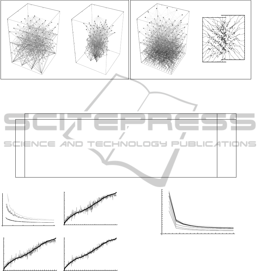
Figure 6: Dendritic structure in the production of digits: (a) ‘3’, and (b) ‘4’, covering layers ℓ from 3 to 5. (c) Cliques of

highly correlated 2-nd layer neurons on the same digits.

0 ® 6

3 ® 8

5 ® 6

6 ® 4

0 ® 0

3 ® 3

5 ® 5

6 ® 6

Figure 5: Examples of incorrectly and correctly classiﬁed

hardly handwritten digits.

works, such as the convergence to a unique output

value, a high sensibility to different initial conﬁgura-

tions, and a poor signiﬁcance of delta-terms in lower

layers (Larochelle et al., 2009).

What is the relevance of the neuron dynamics in

these beneﬁts? Figures 2(b) and (d) show respectively

the ﬁnal layout of the Pumadyn network and the tra-

jectories of the 2-nd and 3-rd layer neurons in the

MNIST experiment. We may observe some notably

layout changes in search of a generally symmetric lo-

cation of downward neurons w.r.t. upward ones, plus

some special features denoting inner encodings. The

latter is precisely a focus of our research. At the mo-

ment, we propose a couple of early considerations.

Thus, in Figures 6(a-b) we capture the typical den-

dritic structure of the most correlated and activenodes

reacting to the features of a digit. Namely, here we

represent only the nodes whose output is signiﬁcantly

far from 0 with high frequency during the processing

of the test set. Then we establish a link between those

neurons, belonging to contiguous layers, which are

highly correlated during the processing of a speciﬁc

digit. An analogous analysis on intra-layer neurons

highlights cliques of neurons jointly highly correlated

in correspondence of the same digit, as shown in Fig-

ure 6(c).

Are these structures relevant? As mentioned in

Section 2, the liaison between the physics and the

cognitive parts of the system is represented by the

penalty factor λ

. Its function is to topologically spe-

cialize the role of the neurons so that the connection

weights decay with the distance between connected

neurons. Thus, an early operational challenge we may

venture is the isolation of a sub-network which main-

tains only informative connections. This goal leads us

to the wide family of pruning algorithms commonly

employed in the literature. In this instance as well, we

may assume that the kinetic morphogenesis we have

implemented, and λ

coefﬁcients in particular, con-

tribute to the emergence of the sub-network as made

up simply of effective connection weights (w

times

) that are tangibly far from 0. For instance, we ex-

perimented that: i) the slimming of the network by

pruning the connections between neurons located at

a distance longer than 20 –with a reduction of 18%

of connections – did not tangibly degrade the regres-

sion accuracy on Pumadyn dataset, at least in a few

instances that we checked; and ii) retraining the net-

work after pruning 50% of the MNIST architecture

did moderately increase the classiﬁcation error rate

from 3.26 to 8%.

5 CONCLUSIONS

In this paper we gained some insights and questions

about a new neural network paradigm. The key mo-

NCTA 2011 - International Conference on Neural Computation Theory and Applications

104

tivation for continuing its exploration stands in the

search of a ground state which takes into account the

agent mobility as a further facility of the neurons. Ac-

tually, artiﬁcial neural networks paradigm borns ex-

actly in view of emulating an analogous paradigm

which proved to be very efﬁcient in nature. Nowadays

we may envisage in social networks an extension of

this paradigm as a social phenomenon which roots a

great part of the ethological system evolution (Easley

and Kleinberg, 2010). In turn, this may be consid-

ered a macro-scale companion of the neuromorphol-

ogy process ruling the early stage of our live. Thus,

we try to transfer one of the main features of both phe-

nomena, namely the agents’ mobility (either actual or

virtual within the web) as a complement to the infor-

mation piping capability of the network connecting

them.

There is a lot of issues related to the task of com-

bining motion with cognitive phenomena. On the one

hand, in a very ambitious perspective we could con-

sider learning as another form of mobility in a proper

subspace, so as to state a link in terms of potential

ﬁelds of the same order scientists stated in the past

between thermodynamic and informative entropy. On

the other hand, we may draw from the granular com-

puting province (Apolloni et al., 2008) the analogous

of the Boltzmann constant (Fermi, 1956) in terms of

links between physical and cognitive aspects. In this

paper, besides the notion of neuron cognitive masses,

we stated this link through the λ coefﬁcients. In turn,

they play a clear role of membership function of the

downward-layer neurons to the cognitive basin of the

upward-layer neurons. We will further elaborate on

these aspects in a future work.

REFERENCES

Apolloni, B., Bassis, S., and Brega, A. (2009). Feature se-

lection via Boolean Independent Component analysis.

Information Science, 179(22):3815–3831.

Apolloni, B., Bassis, S., Malchiodi, D., and Pedrycz, W.

(2008). The Puzzle of Granular Computing, volume

138. Springer Verlag.

Carpenter, G. A. and Grossberg, S. (2003). Adaptive reso-

nance theory. In The Handbook of Brain Theory and

Neural Networks, pages 87–90. MIT Press.

Ciresan, D. C., Meier, U., Gambardella, L. M., and Schmid-

huber, J. (2010). Deep big simple neural nets for

handwritten digit recognition. Neural Computation,

22(12):3207–3220.

Corke, P. I. (1996). A robotics toolbox for Matlab. IEEE

Rob. and Aut. Mag., 3(1):24–32.

Danafar, S., Gretton, A., and Schmidhuber, J. (2010).

Characteristic kernels on structured domains excel in

robotics and human action recognition. In Machine

Learning and Knowledge Discovery in Databases,

volume 6321, pages 264–279. Springer, Berlin.

Dirac, P. A. M. (1982). The Principles of Quantum Mechan-

ics. Oxford University Press, USA.

Easley, D. and Kleinberg, J. (2010). Networks, Crowds,

and Markets: Reasoning About a Highly Connected

World. Cambridge University Press, Cambridge, MA.

Ezhov, A. and Ventura, D. (2000). Quantum neural net-

works. Future Directions for Intelligent Systems and

Information Science 2000.

Fermi, E. (1956). Thermodynamics. Dover Publications.

Feynman, R., Leighton, R., and Sands, M. (1963). The

Feynman Lectures on Physics, volume 3. Addison-

Wesley, Boston.

Hinton, G. E., Osindero, S., and Teh, Y. W. (2006). A fast

learning algorithm for deep belief nets. Neural Com-

putation, 18:1527–1554.

Kreutz-Delgado, K. and Rao, B. D. (1998). Application

of concave/Schur-concave functions to the learning of

overcomplete dictionaries and sparse representations.

In 32th Asilomar Conference on Signals, Systems &

Computers, volume 1, pages 546–550.

Larochelle, H., Bengio, Y., Louradour, J., and Lamblin, P.

(2009). Exploring strategies for training deep neural

networks. Jour. Machine Learning Research, 10:1–40.

LeCun, Y. (1988). A theoretical framework for back-

propagation. In Proc. of the 1988 Connectionist Mod-

els Summer School, pages 21–28. Morgan Kaufmann.

LeCun, Y., Bottou, L., Bengio, Y., and Haffner, P. (1998).

Gradient-based learning applied to document recogni-

tion. Proceedings of the IEEE, 86(11):2278–2324.

Mar´ın, O. and Lopez-Bendito, G. (2007). Neuronal migra-

tion. In Evolution of Nervous Systems: a Comprehen-

sive Reference, chapter 1.1. Academic Press.

Mar´ın, O. and Rubenstein, J. L. (2003). Cell migration in

the forebrain. Review in Neurosciences, 26:441–483.

NVIDIA Corporation (2010). Nvidia Tesla c2050 and

c2070 computing processors.

Rasmussen, C. E., Neal, R. M., Hinton, G. E., van Camp,

D., Revow, M., Ghaharamani, Z., Kustra, R., and

Tibshirani, R. (1996). The Delve manual. Techni-

cal report, Dept. Computer Science, Univ. of Toronto,

Canada. Ver. 1.1.

Stanley, K. O. and Miikkulainen, R. (2002). Evolving neu-

ral networks through augmenting topologies. Evolu-

tionary Computation, 10(2):99–127.

KINETIC MORPHOGENESIS OF A MULTILAYER PERCEPTRON

105