
UNSUPERVISED HANDWRITTEN GRAPHICAL SYMBOL
LEARNING
Using Minimum Description Length Principle on Relational Graph
Jinpeng Li, Harold Mouchere and Christian Viard-Gaudin
IRCCyN (UMR CNRS 6597), L’UNAM, Universit´e de Nantes, Nantes, France
Keywords:
Unsupervised graphical symbol learning, Graph mining, Minimum description length principle, Online hand-
writing.
Abstract:
Generally, the approaches encountered in the field of handwriting recognition require the knowledge of the
symbol set, and of as many as possible ground-truthed samples, so that machine learning based approaches
can be implemented. In this work, we propose the discovery of the symbol set that is used in the context of
a graphical language produced by on-line handwriting. We consider the case of a two-dimensional graphical
language such as mathematical expression composition, where not only left to right layouts have to be consid-
ered. Firstly, we select relevant graphemes using hierarchical clustering. Secondly, we build a relational graph
between the strokes defining an handwritten expression. Thirdly, we extract the lexicon which is a set of graph
substructures using the minimum description length principle. For the assessment of the extracted lexicon, a
hierarchical segmentation task is introduced. From the experiments we conducted, a recall rate of 84.2% is
reported on the test part of our database produced by 100 writers.
1 INTRODUCTION
In different physical aspects of language (textual lan-
guage, graphical language, etc.) the knowledge of the
symbol set is of paramount importance. In this paper,
we are working on an online handwritten graphical
language. Most of the existing recognition systems
dedicated to graphical languages, if not all, need the
definition of the character or symbol set. Then, they
require a training dataset which defines the ground-
truth at the symbol level so that a machine learning
algorithm can be trained on this task to recognize
symbols from handwritten information. Many recog-
nition systems take advantage from the creation of
large, realistic corpora of ground-truthed data. Such
datasets are valuable for the training, evaluation, and
testing stages of the recognition systems in different
domains. They also allow comparison between state-
of-the-art recognizers. However, collecting all the ink
samples and labelling them at the stroke level is a very
long and tedious task. Hence, it would be very inter-
esting to be able to assist this process, so that most
of the tedious work can be done automatically, and
that only a high level supervision need to be defined
to conclude the labelling process.
In this respect, we propose to extract automati-
cally the relevant patterns which will define the lex-
ical units of the language. This process is carried out
from the redundancy in appearance of basic regular
shapes and regular layout of these shapes in a large
collection of handwritten scripts.
These handwritten scripts derive from a language.
In other words, a language, which uses a set of rules,
generates some handwritten scripts (observations).
For the terminology, we use the word “evidences” for
the observations from a language (Marcken, 1996b).
A language could be Context Free Grammar (CFG)
generator (Solan et al., 2005), but certainly the human
natural language is more complex than CFG (Chom-
sky, 1956). On textual corpora, which can be consid-
ered as a subform of simple graphical languages, un-
supervised learning of CFG has been discussed and
considered as a non-trivial task (Alexander Clark and
Lappin, 2010; Carroll et al., 1992; Gold, 1967). We
propose to extend this kind of approach on real graph-
ical languages where not only left to right layouts
have to be considered.
To tackle this problem, most of the works are us-
ing heuristic approaches (Alexander Clark and Lap-
pin, 2010). One of the famous approaches is the Mini-
mum Description Length (MDL) principle (Rissanen,
1978) which assumes that the best lexicon minimizes
172
Li J., Viard-Gaudin C. and Mouchere H..
UNSUPERVISED HANDWRITTEN GRAPHICAL SYMBOL LEARNING - Using Minimum Description Length Principle on Relational Graph.
DOI: 10.5220/0003637901640170
In Proceedings of the International Conference on Knowledge Discovery and Information Retrieval (KDIR-2011), pages 164-170
ISBN: 978-989-8425-79-9
Copyright
c
2011 SCITEPRESS (Science and Technology Publications, Lda.)

the description length of lexicon and of evidences us-
ing the extracted lexicon. Using this MDL principle, a
recall rate of 90.5% for symbols is reported (Marcken,
1996a) on the Brown English corpus, (Francis and
Kuˇcera, 1982). In fact, (Marcken, 1996a) extracted
a hierarchical lexicon which could be considered as a
CFG where the symbols are the elements in lexicon.
In this paper, the application domain is online
handwriting. On a online graphical corpus, the
units (strokes) are composed in evidences with two-
dimensional spatial relations. In this case, the search
space for the combination of units which makes up
possible lexical units is much more complex since
it is no longer a linear one. We can describe these
two-dimensional spatial relations with a graph. Thus
a graph mining technique is required to extract the
repetitive pattern on the graph. Such a task is per-
formed with the SUBDUE (SUBstructure Discovery
Using Examples) system (Cook and Holder, 2011). It
is a graph based knowledge discovery method which
extracts the substructures in a graph using MDL prin-
ciple.
This paper proposes a solution for the mod-
elling of a two-dimensional graphical language with
a graph. Then, using SUBDUE, the lexicon is ex-
tracted, we also study how to evaluate the extracted
lexicon in terms of symbol-based ground-truths. We
give an overview of the proposed system in section
2. Then, the design of the relational graph from the
evidences produced by a given graphical language,
the extraction of lexicon using the system SUBDUE
based on the relational graph and the evaluation of
the extracted lexicon are discussed in section 3, be-
fore presenting the experimental results in section 4.
2 OVERVIEW
In this section, we give an overview of the proposed
method for extracting graphical symbols (lexicon)
from a handwriting corpus as shown in Figure 1. We
use three principal steps: i) quantization of strokes
into grapheme prototypes, ii) construction of rela-
tional graphs between strokes and, iii) extraction of
the lexicon composed of graphemes and spatial rela-
tions.
As shown in Figure 1, given a new graphical
language, we are firstly interested in finding the
graphemes, which represent the different possible
shapes of strokes. A clustering technique is used
for generating a finite set of these graphemes (code-
book). Then, the quantization step consists of using
this codebook to tag all the strokes. Secondly, the
spatial relations between strokes are extracted for or-
ganizing a relational graph inspired by the Symbol
Relation Tree approach (SRT) (Rhee and Kim, 2009).
Thirdly, we extract the repetitive patterns as lexical
units in the relational graph using Minimum Descrip-
tion Length (MDL) principle (Rissanen, 1978; Cook
and Holder, 1994). We could consider these lexical
units as the symbols.
Handwriting
database
2
3
|
8
Graphemes
1.Quantization
Relational graphs
Lexical unit
B
=
B
:Below
:Grapheme
2.Construction of relational graphs
3.Lexicon extraction
Clustering
2
3
8
|
|
8
(1)
(2)
(3)
(4)
(5)
(6)
(7)
(8)
(9)
(12)
(12)
(13)
(14)
(15)
(1)
(2)
(3)
(4)
(5)
(9)
(8)
(12)
(6)
(10)
(12)
(14)
(15)
B
(4)
B
(5)
(11)
(12)
|
(7)
(10)
(13)
Figure 1: Overview for unsupervised graphical symbol
learning.
As an example in Figure 1, we assume a handwrit-
ing database containing two handwritten expressions
“8− 3 = 8” and “1 ± 2 = 4”. Each stroke is marked
by the index (.) to avoid ambiguity. The following
set of graphemes { ‘3’,‘∠ ’, ‘−’,‘2’,‘8’,‘|’} defining
the codebook may be found. To obtain it, an unsu-
pervised clustering algorithm is used. Then, we code
each stroke using this codebook. This is the quantiza-
tion step. Afterwards, we analyse the spatial relations
between two different strokes to organize a relational
graph. There are many spatial relations between two
different strokes in the database. As a simple exam-
ple, the frequent substructure ( ‘−’
B
→
‘−’ ) could be
discovered from the relational graph. This substruc-
ture means that a stroke represented by a grapheme
‘−’ is found below another stroke coded by the same
grapheme ‘−’. We could consider this substructure as
a lexical unit. In that case, this lexical unit represents
the operator equal (‘=’).
We mainly focus in this work on the problem of
building a relational graph with a reasonable com-
plexity, then extracting a lexicon from this graph and
evaluating our lexicon using a hierarchical segmenta-
tion task.
3 UNSUPERVISED GRAPHICAL
SYMBOL LEARNING
To discover graphical symbols, we firstly extract the
UNSUPERVISED HANDWRITTEN GRAPHICAL SYMBOL LEARNING - Using Minimum Description Length
Principle on Relational Graph
173

graphemes from strokes using a hierarchical cluster-
ing. After the quantization of each stroke, a rela-
tional graph is then generated for modelling spatial
relations between strokes. To minimize the descrip-
tion length of the relational graph, an algorithm (Cook
and Holder, 1994) is applied to discover the repetitive
substructures which are probably the lexical units.
3.1 Quantization of Strokes
The data that we are interested in are online hand-
writing, available as sequences of strokes, which
are themselves sequences of 2D points. Because of
the variability of shapes produced by handwriting,
we need to quantify the strokes into a finite set of
graphemes (codebook). We measure the dissimilar-
ity between two shapes of strokes using a Dynamic
Time Warping (DTW) algorithm (Vuori, 2002). Clus-
tering techniques are used for producing the code-
book. Instead of using a traditional k-means algo-
rithm which is prone to initialisation problems, we
prefer an agglomerative hierarchical clustering since
the tree topology is favourable to tune easily the num-
ber of prototypes. Once the number of n
p
graphemes
(the final prototypes of hierarchical clustering) is se-
lected, all the strokes are tagged with the virtual label
of the closest grapheme. This procedure is the quan-
tization of strokes. Afterwards, we build relational
graphs between strokes.
3.2 Construction of Relational Graphs
This section presents the construction of the rela-
tional graph inspired by SRT (Rhee and Kim, 2009).
We define the nodes as the strokes labelled with its
grapheme prototype (one of the codebook element)
and the edges as a spatial relation. We define a spa-
tial relation as a relationship from a reference stroke
to an argument stroke. In other words, the relational
graph is directed. This allows for instance to distin-
guish between the two following horizontal layout of
two graphemes: “−|” or “|−”, which are two differ-
ent symbols. Concerning the complexity, suppose we
have n
r
different spatial relations and n
str
different
strokes, to create a complete directed graph for all the
vertices (strokes), the number of directed edges is
2·n
r
C
2
n
str
= n
r
n
str
(n
str
− 1) (1)
where C
m
n
=
n(n−1)...(n− m+1)
m(m−1)...2·1
(Chartrand, 1985). In
that case, the search space would be far more too com-
plex to search patterns in the complete directed graph.
Therefore, the number of out-directed edges from a
referencestroke should be limited to n
c
closest strokes
where n
c
<= n
str
− 1 since we, human, have a limited
perceived visual angle (Baird, 1970); we prefer some
symbols composed of the closest strokes. Therefore,
the reduced number of directed edges is:
n
r
· n
str
· n
c
. (2)
However, if n
c
is too small, we could lose some sym-
bols. In our work, we select three spatial relations
n
r
= 3, namely, right (R), below (B) and intersection
(I). We consider relation I having a higher priority
than directional relations, R and B. In other words, I
is exclusive with R and B. This constraint means that
if two strokes are intersected, we do not consider the
directional relationships but only the topological rela-
tionships between two spatial objects (Schneider and
Behr, 2006). It turns out that the maximum number of
directed edges is:
2·n
str
· n
c
(3)
since the maximum outdegree of reference stroke is
two. To reduce even more the number of edges of this
relational graph, we constrain the graph construction
to obtain a Directed Acyclic Graph (DAG). We start
with the top-left stroke to initiate the DAG. Then from
a reference stroke, we explore the three possible spa-
tial relations (R, B and I) to find the next possible
strokes but without considering the strokes already
used from the starting stroke to the reference stroke.
At the end, since I is a symmetric spatial relation, we
add one more edge from the argument stroke to the
reference stroke for I. Considering Eq.(2), the maxi-
mum n
r
is still 2 since I is symmetric and is exclusive
with R and B. Therefore, we reduced the search space
significantly.
As an example, Figure 2 illustrates a simple math-
ematical expression “1± 2 = 4”. When we consider
the stroke (6) coded by the grapheme ‘−’ as the refer-
ence stroke, the search for the n
c
= 2 closest strokes to
create the relational graph is shown in Figure 2. Right
and below projection areas of ‘−
(6)
’ (see the shadow
areas in Figure 2) are applied for detecting the next
strokes.
Reference stroke
(8)
(7)
(9)
(5)
(6)
Right
Below
(.) : Indices of stroke
Bounding box for all strokes
(1)
(2)
(3)
(4)
Figure 2: Two directional relations (right and below) in
terms of the reference stroke −
(6)
.
The corresponding sub-graph with reference node
‘−
(6)
’ is shown in Figure 3 using n
c
= 2 closest next
KDIR 2011 - International Conference on Knowledge Discovery and Information Retrieval
174

B
(7)
(6)
(9)(8)
R
R
B : Below
R : Right
(.) : Indices of stroke
: Graphemes
Figure 3: Search spatial relations using n
c
= 2 closest
strokes from the reference stroke (6) with grapheme ‘−’.
strokes. ‘∠
(8)
’ and ‘|
(9)
’ are right of ‘−
(6)
’, and ‘−
(7)
’
is found below ‘−
(6)
’.
To create the relational graph for the full expres-
sion “1± 2 = 4” using n
c
= 2, we start with the top-
left stroke ‘|
(1)
’ as shown in Figure 4. We can see that
the operator “±” (‘−
(2)
’
I
⇄
I
‘|
(3)
’
B
→
‘−
(4)
)’), the op-
erator “=” (‘−
(6)
’
B
→
‘−
(7)
’) and the digit “4” (‘∠
(8)
’
I
⇄
I
‘|
(9)
’) are actually present in the relational graph.
(2)
(4)
R
R
(1)
(8)
R
(3)
I
I
B
2
(5)
R
(6)
(7)
R
R
R
R
(9)
R
R
R
R
I
I
B
B: Below
R: Right
(.) : Indices of stroke
: Graphemes
Figure 4: Generated relational graph using n
c
= 2 closest
strokes for the expression “1± 2 = 4” from Figure 2.
If we had created a complete directed relational
graph for 9 strokes using 3 different spatial relations,
the number of edges would be using Eq. (1) 3·9·(9−
1) = 216. After pruning, the maximum of number of
edges is 2 · 9 · 2 = 36 using Eq. (3) where n
c
= 2.
The number of edges is much smaller than that of the
complete directed graph. With the constraint of DAG
and with an additional edge for I, 18 directed edges
are created as shown in Figure 4.
In this section, we have shown how to build a rela-
tional graph for a graphical language. As an example,
we have used a simple expression to show the cre-
ation of this relational graph. In the next section, we
will see how to extract the repetitive hierarchical sub-
structures (sub-graphs)from the relational graph. The
set of repetitive hierarchical substructures is probably
composing the lexicon (i.e. the set of symbols used in
the language).
3.3 Lexicon Extraction using Minimum
Description Length Principle on
Relational Graph
In previous section, we get the relational graph for
a graphical language. This section presents an al-
gorithm from (Cook and Holder, 1994) using Min-
imum Description Length (MDL) principle (Rissa-
nen, 1978) to extract repetitive substructures in graph,
which will be considered in our context as the lexical
units. In unsupervised language learning model, the
MDL principle implies that the best lexical unit min-
imize the description length of both the lexical unit
and of the graph using lexical unit(Marcken, 1996b).
Formally given a graph G, we try to choose the lexical
unit u which minimize the description length
DL(G, u) = I(u) + I(G|u) (4)
where I(u) is the number of bits to encode the lex-
ical unit u and I(G|u) is the number of bits to en-
code the graph G using the lexical unit u. (Cook and
Holder, 1994) give the precise definition of DL(G, u).
The system SUBDUE (SUBstructure Discovery Us-
ing Examples) (Cook and Holder, 2011) extracts it-
eratively the best lexical unit (substructure) using
(MDL) principle. A unit could be a hierarchical struc-
ture (Jonyer et al., 2000).
For explaining the iterative procedure and the hi-
erarchical structure, we use the same example of ex-
pression “1 ± 2 = 4”, which contains a hierarchical
structure “±” shown in Figure 4. Obviously, this ex-
pression has to be part of a training expression set
which allows to compute frequency of possible lex-
ical units. We assume that there are many instances
of “=” in the training set. Probably we could discover
the lexical unit LU 1 (“=”) in first iteration. Then we
could extract another frequent lexical unit LU 2 (“4”)
in the second iteration, and frequent lexical unit LU 3
(“+”) in a third iteration. LU i designates a discov-
ered lexical unit in i
th
iteration, as shown in Figure
5. A lexical unit corresponds to different instances in
the graph. For example, LU 1 has one instance in the
relational graph in Figure 5.
:Instance of a discovered lexical unit
(2)
(4)
R
R
(1)
(8)
B: Below
R: Right
(.) : Indices of stroke
: Graphemes
R
(3)
I
I
B
2
(5)
R
(6)
(7)
R
R
R
R
(9)
R
R
R
R
I
I
B
LU_1
LU_2
LU_3
Figure 5: Three discovered lexical units LU 1, LU 2 and
LU 3 in first, second and third iteration.
UNSUPERVISED HANDWRITTEN GRAPHICAL SYMBOL LEARNING - Using Minimum Description Length
Principle on Relational Graph
175

Therefore, we replace all the instances of lexi-
cal unit with the lexical unit’s name in the relational
graph. Figure 6 shows the new relational graph using
LU 1, LU 2 and LU 3 ready for the fourth iteration.
In the fourth iteration, the lexical unit LU 4 would
be probably extracted. LU 4 contains LU 3 which
means that LU 4 is a hierarchical structure. The index
(.) of LU 1, LU 2, and LU 3 for strokes are deleted
since there are many strokes corresponding to only
one lexical unit in Figure 6.
|
I
|
I
LU_3:
LU_2:
I
I
{(2),(3)}
(4)
R
R
(1)
R
B
2
(5)
R
{(6),(7)}
R
R
R
R
{(8),(9)}
R
R
R
R
LU_1
LU_2
LU_3
B
LU_1:
LU_4
:Instance of a discovered lexical unit
B: Below
R: Right
(.) : Indices of stroke
: Graphemes
Figure 6: A discovered lexical unit LU 4 are extracted in
fourth iteration.
Figure 7 shows the extracted hierarchical lexicon
(extracted substructures) when no more lexical unit
can reduce the description length. In other words, the
lexicon are the list of lexical units L =(LU 1, LU 2,
LU 3,...) in terms of DL(G, u).
{(2),(3),(4)}
R
R
(1)
R
2
(5)
R
{(6),(7)}
R
R
R
R
{(8),(9)}
R
R
R
R
LU_1
LU_2
LU_4
:Instance of a discovered lexical unit
B: Below
R: Right
(.) : Indices of stroke
: Graphemes
|
I
LU_2:
B
LU_1:
B
LU_4:
LU_3
|
I
LU_3:
I
Figure 7: A hierarchical extracted lexicon at the end of iter-
ation.
At the end, we extract a sorted list of lexical units
from the relational graphs using MDL principle. We
call this list of lexical units as lexicon. In next sec-
tion, we evaluate the extracted lexicon using a task of
hierarchical segmentation of new graphical evidences
from the same graphical language.
3.4 Evaluation
We extracted the lexicon which is a sorted list of sub-
structures L =(LU 1, LU 2, LU 3,...). Given some
new graphical evidences e from the same graphical
language which has generated the lexicon, we inter-
pret these evidences by a simple task of bottom-up
combination which produces a hierarchical segmen-
tation by SUBDUE (Cook and Holder, 2011). Firstly,
we build the relational graph for the evidences. Sec-
ondly, SUBDUE replaces all the instances in the rela-
tional graph with lexical units from LU 1 to the end of
the sorted list since the lexical units are sorted using
description length. Finally, we can get a hierarchical
segmentation S(e, L).
In order to evaluate the segmentation, we use four
measures (LI et al., 2011; Marcken, 1996b) which are
applied in graphical language learning: R
Recall
, R
CB
,
R
Top
, and R
CB
. The recall rate R
Recall
evaluates the
percentage of right segmentation which are found in
ground-truths. On the contrary the second measure
R
CB
reveals the error of the segmentation compared
with ground-truths. The third measure is defined by
R
Lost
= 1 − R
Recall
− R
CB
. Moreover R
Top
evaluates
the performance of longest possible segments of the
hierarchical segmentation. R
Top
is the same definition
of R
Good
in (LI et al., 2011). In next section, we create
an artificial database to evaluate the method.
4 SEGMENTATION
EXPERIMENTS
We firstly introduce a handwriting database to eval-
uate our approach. Using the hierarchical segmenta-
tion and the presented measures, the extracted lexicon
is secondly evaluated in terms of different numbers of
prototypes.
To test the performance of our approach, we cre-
ated an artificial database named Calculate (LI et al.,
2011; Awal, 2010) of realistic handwritten expres-
sions from isolated symbols. Firstly the expressions
in Calculate are generated in terms of the grammar
N
1
op N
2
= N
3
where N
1
, N
2
and N
3
are numberscom-
posed of 1, 2 or 3 digits from {0, 1, ...,9}. The distri-
bution of number of digits for N
i={1,2,3}
is 70% of 1
digit, 20% of 2 digits and 10% of 3 digits randomly.
In addition, op represents the operators {+, −, ×, ÷}.
Figure 8 shows an example in Calculate with N
1
, N
2
,
N
3
and op containing 3 digits, 1 digit, 2 digits and “×”
respectively. Secondly Calculate is separated into a
training part and a test part. The training part con-
tains 897 expressions from 180 writers for the un-
supervised learning. On this part we computed the
graphemes by clustering and extracted the lexicon
by the iterative search algorithm. The test part con-
tains 497 expressions written by another 100 writers.
Learned graphemes and lexicon are tested on this part.
We extract the lexicon on the training part of Cal-
culate in terms of different numbers of prototypes on
the training part using n
c
= 2 and evaluate the ex-
KDIR 2011 - International Conference on Knowledge Discovery and Information Retrieval
176
N
1
N
2
N
3
op =
Figure 8: A synthetic expression from the Calculate
database.
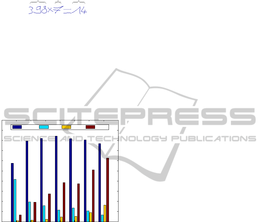
tracted lexicon on the test part shown in Figure 9.
We obtain the best R
Recall
= 84.2% (R
CB
= 11.3%,
R
Lost
= 4.5% and R
Top
= 38.3%) using n
p
= 120
on the test part. The increasing number of proto-
types increases the performance of R
Top
while R
Recall
almost remains unchanged starting from n
p
= 30
since it exists many symbols composed of only one
stroke. Comparing with the recall rate of 90.5% us-
ing MDL principle in (Marcken, 1996a; Marcken,
1996b) on Brown corpus (sequences of ASCII char-
acters)(Francis and Kuˇcera, 1982), our recall rate of
84.2% on test part is fair.
15 30 75 120 150 225 300
0
0.1
0.2
0.3
0.4
0.5
0.6
0.7
0.8
0.9
1
RecallRate CBRate LostRate TopRate
Figure 9: Extraction of the lexicon in terms of different
numbers of prototypes using n
c
= 2 on training part and
its evaluation of extracted lexicon on test part.
5 CONCLUSIONS
In this paper, we study an unsupervised learning prob-
lem to extract the graphical symbols in a graphical
language. Firstly, we extract the graphemes using hi-
erarchical clustering and quantify the strokes using
the extracted graphemes. Secondly, we discuss how
to create a relational graph to simplify the complex-
ity of learning. Thirdly, using the system SUBDUE,
we extract the lexicon with MDL principle. To eval-
uate the extracted lexicon, several measures are in-
troduced. At the end, we get a recall rate of 84.2%
on the test part of our synthetic database. However,
this database only contains one-line mathematical ex-
pressions whose spatial relations are relative sim-
ple. Some more complex graphical languages, e.g.
flowcharts or complex mathematical expressions, are
still needed to be studied. More complex spatial re-
lations would be our future work. Furthermore, some
criteria to stop earlier the iterative learning algorithm
and to find the right number of prototypes should be
explored.
ACKNOWLEDGEMENTS
This work is supported by the French R´egion Pays
de la Loire in the context of the DEPART project
www.projet-depart.org.
REFERENCES
Alexander Clark, C. F. and Lappin, S. (2010). The Hand-
book of Computational Linguistics and Natural Lan-
guage Processing. Wiley-Blackwell.
Awal, A. M. (2010). Reconnaissance de struc-
tures bidimensionnelles: Application aux expres-
sions math´ematiques manuscrites en-ligne. PhD the-
sis, Ecole polytechnique de l’universit´e de Nantes,
France.
Baird, J. C. (1970). Psychophysical analysis of visual space.
Oxford, London: Pergamon Press.
Carroll, G., Carroll, G., Charniak, E., and Charniak, E.
(1992). Two experiments on learning probabilistic de-
pendency grammars from corpora. In Working Notes
of the Workshop Statistically-Based NLP Techniques,
pages 1–13. AAAI.
Chartrand, G. (1985). Introductory Graph Theory. Dover
Publications.
Chomsky, N. (1956). Three models for the description of
language. IRE Transactions on Information Theory,
2:113–124.
Cook, D. J. and Holder, L. B. (1994). Substructure dis-
covery using minimum description length and back-
ground knowledge. J. Artif. Int. Res., 1:231–255.
Cook, D. J. and Holder, L. B. (2011). Substructure discov-
ery using examples. http://ailab.wsu.edu/subdue/.
Francis, N. W. and Kuˇcera, H. (1982). Frequency Analysis
of English Usage: Lexicon and Grammar., volume 18.
Houghton Mifflin, Boston.
Gold, E. M. (1967). Language identification in the limit.
Information and Control, 10(5):447–474.
Jonyer, I., Holder, L. B., and Cook, D. J. (2000). Graph-
based hierarchical conceptual clustering. Interna-
tional Journal on Artificial Intelligence Tools, 2:107–
135.
Li, J., Mouchere, H., and Viard-Gaudin, C. (2011). Sym-
bol knowledge extraction from a simple graphical lan-
guage. In ICDAR2011.
UNSUPERVISED HANDWRITTEN GRAPHICAL SYMBOL LEARNING - Using Minimum Description Length
Principle on Relational Graph
177

Marcken, C. D. (1996a). Linguistic structure as composi-
tion and perturbation. In In Meeting of the Association
for Computational Linguistics, pages 335–341. Mor-
gan Kaufmann Publishers.
Marcken, C. D. (1996b). Unsupervised Language Acquisi-
tion. PhD thesis, Massachusetts Institute of Technol-
ogy.
Rhee, T. H. and Kim, J. H. (2009). Efficient search
strategy in structural analysis for handwritten math-
ematical expression recognition. Pattern Recognition,
42(12):3192 – 3201.
Rissanen, J. (1978). Modeling by shortest data description.
Automatica, 14(5):465 – 471.
Schneider, M. and Behr, T. (2006). Topological relation-
ships between complex spatial objects. ACM Trans.
Database Syst., 31:39–81.
Solan, Z., Horn, D., Ruppin, E., and Edelman, S. (2005).
Unsupervised learning of natural languages. PNAS,
102(33):11629–11634.
Vuori, V. (2002). Adaptive Methods for On-Line Recogni-
tion of Isolated Handwritten Characters. PhD thesis,
Helsinki University of Technology (Espoo, Finland).
KDIR 2011 - International Conference on Knowledge Discovery and Information Retrieval
178
