CASCADE OF MULTI-LEVEL MULTI-INSTANCE
CLASSIFIERS FOR IMAGE ANNOTATION
Cam-Tu Nguyen
1
, Ha Vu Le
2
and Takeshi Tokuyama
1
1
Graduate School of Information Sciences, Tohoku University, Sendai, Japan
2
VNU University of Engineering and Technology, Hanoi, Vietnam
Keywords:
Image annotation, Cascade algorithm, Multi-level feature extraction.
Abstract:
This paper introduces a new scheme for automatic image annotation based on cascading multi-level multi-
instance classifiers (CMLMI). The proposed scheme employs a hierarchy for visual feature extraction, in
which the feature set includes features extracted from the whole image at the coarsest level and from the
overlapping sub-regions at finer levels. Multi-instance learning (MIL) is used to learn the “weak classifiers” for
these levels in a cascade manner. The underlying idea is that the coarse levels are suitable for background labels
such as “forest” and “city”, while finer levels bring useful information about foreground objects like “tiger”
and “car”. The cascade manner allows this scheme to incorporate “important” negative samples during the
learning process, hence reducing the “weakly labeling” problem by excluding ambiguous background labels
associated with the negative samples. Experiments show that the CMLMI achieve significant improvements
over baseline methods as well as existing MIL-based methods.
1 INTRODUCTION
Only after a couple of years, online photo-sharing
websites (Flickr, Picassa web, Photobucket, etc.),
which host hundreds of millions of pictures, have
quickly become an integral part of the Internet. As
a result, the need for tagging images and multimedia
data with semantic labels becomes increasingly im-
portant in order to make the Web more well-organized
and accessible. On the other hand, the enormous
amount of photos taken everyday makes the task of
manual annotation an extremely time-consuming and
expensive task. Automatic image annotation there-
fore receives significant interest in image retrieval and
multimedia mining.
Although image classification and object recogni-
tion also assign meta data to images, the difference
of image annotation from classification and recogni-
tion defines its typical challenging issues. In gen-
eral, the number of labels (classes/objects) is usually
larger in image annotation compared to classification
and recognition. Because of the dominating number
of negative examples, both the one-vs-one and one-
vs-all schemes in multi-class supervised learning do
not scale very well for image annotation. Unlike ob-
ject recognition, image annotation is “weakly label-
ing” (Carneiro et al., 2007), that is a label is assigned
Level 1 Level 2
Level 3
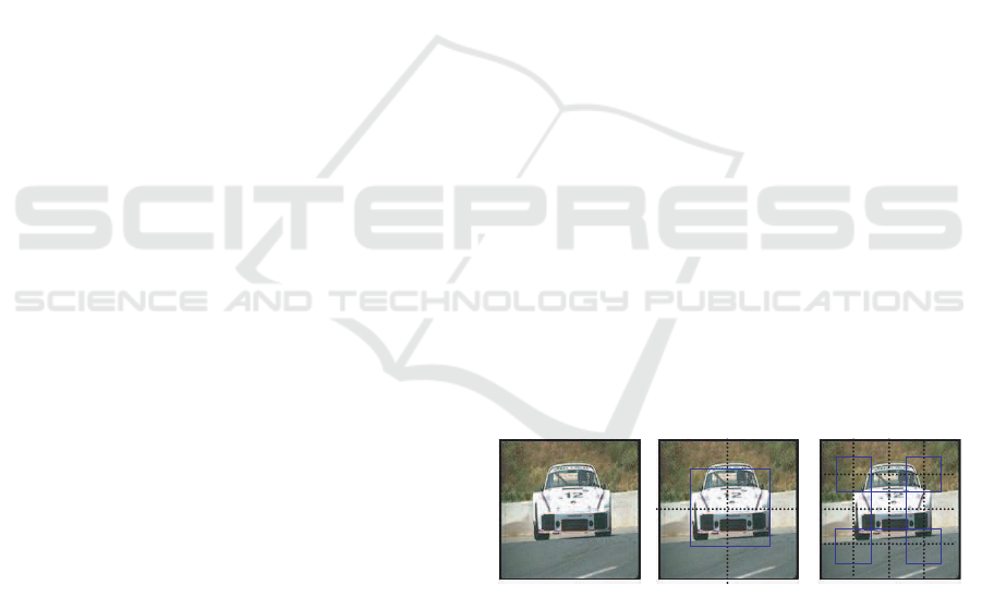
Figure 1: Level 1: the whole image; Level 2: 2x2 grid + 1
subregion in the center; Level 3: 4x4 grid + 5 overlapping
subregions (blue border rectangles).
to one image without indication of the region corre-
sponding to that label. Moreover, scalability require-
ment prevents researchers to investigate feature ex-
traction for every label in image annotation. This,
however, can be performed with a limited number of
objects in object recognition . On the other hand, the
variety of visual representations of objects suggests
that we should not depend on one feature extraction
method to work well with a large number of labels
(Akbas and Vural, 2007; Makadia et al., 2010).
Motivated by the aforementioned issues, we pro-
pose a new learning method - a cascade of multilevel
multi-instance classifiers (CMLMI) for image anno-
tation. The idea behind our approach is that coarser
levels provide better description for background and
common concepts such as “forest, building, moun-
14
Nguyen C., Le H. and Tokuyama T..
CASCADE OF MULTI-LEVEL MULTI-INSTANCE CLASSIFIERS FOR IMAGE ANNOTATION.
DOI: 10.5220/0003634400140023
In Proceedings of the International Conference on Knowledge Discovery and Information Retrieval (KDIR-2011), pages 14-23
ISBN: 978-989-8425-79-9
Copyright
c
2011 SCITEPRESS (Science and Technology Publications, Lda.)

tain”, while finer levels bring useful information to
specific objects such as “tiger, cars, bear”. Given an
object, the cascade method ensures that we first detect
the object’s related scene, then focus on the “likely”
scene to further recognize the object in that context.
Formally, cascading means that learning classifiers
at finer levels (e.g. level 3) is dependent of classi-
fiers at coarser levels (e.g. level 1,2) (learning from
coarse-to-fine). By so doing, when learning classi-
fiers for specific objects at finer levels, we can ignore
(negative) samples of non-related scenes, thus reduce
training time. Since negative examples are those of
the same scene without the considered object, there
is more chance for us to separate the object from the
background. For instance, since a “tiger” usually ap-
pears in a forest, the negative examples of forest back-
ground, which does not contain “tiger”, helps recog-
nize “negative”regions (forest regions) in the positive
examples of “tiger”. As a result, it improvesthe selec-
tion of regions corresponding to “tiger”, and reduces
the ambiguity of “weakly labeling”.
Specifically, our propose contains two main parts:
1) multi-level feature extraction; and 2) cascade of
multi-instance classifiers over multiple levels. Multi-
level means we divide images into different levels of
granularity from the coarsest one (the whole image) to
increasingly fine subregions (Figure 1). Several fea-
ture extraction algorithms are performed at each level,
each algorithm produces a set of feature vectors cor-
responding to subregions of the image. Given a label,
a cascade of multi-level multi-instance classifiers is
then built across levels, from cheapest (coarsest) fea-
tures to the most expensive (finest) features. Here,
features extracted from the whole image (level 1) are
called global features.
In the literature, cascade of classifiers were suc-
cessfully used to design fast object detectors (Viola
and Jones, 2001) while multi-level features were ap-
plied to image classification (Lazebnix et al., 2009)
and object recognition (Torralba et al., 2010). To the
best of our knowledge, however, this is one of the first
attempts that adopts the hierarchy of multi-level fea-
ture extraction to group features according to acqui-
sition cost so as to develop a cascade learning algo-
rithm for image annotation. In comparison with pre-
vious cascading algorithms, we take into account the
“weakly labeling” problem by using MIL and make
the cascading algorithm suitable to image annotation.
In addition, our approach is more robust than previous
MIL methods because we consider multi-level feature
extraction which allows us to cope with the variety in
visual representation among labels. The advantages,
thus, lie in threefold: 1) reducing training time by a
cascade learning algorithm; 2) relaxing the ambiguity
of “weakly labeling” problem of image annotation;
and 3) obtaining strong classifiers, which are robust
to multiple resolution.
The rest of this paper is organized in 6 sections.
Section 2 summarizes typical approachesto image an-
notation and related tasks. Multi-level feature extrac-
tion and multi-instance learning are presented in Sec-
tion 3 and Section 4. Our proposed method for image
annotation is givenin details in Section 5. Experimen-
tal results will be given in Section 6. Finally, Section
7 concludes the important remarks of our work.
2 RELATED WORKS
Image annotation and related tasks (object recogni-
tion, image classification and retrieval) have been the
active topics for more than a decade and led to sev-
eral noticeable methods. In the following, we present
an overview of typical approaches, which are cate-
gorized into 1) classification-based methods; and 2)
joint-distribution based methods.
2.1 Classification-based Approach
The early effort in the area is to formalize image anno-
tation as the task of binary classification. Some exam-
ples are to classify images into “indoor” or “outdoor”
(Szummer and Picard, 1998). In object recognition,
Viola and Jones (Viola and Jones, 2001) proposed a
method for face detection (face/non face classifica-
tion) using Adaboost, which is very fast in dropping
non face windows in images, thus results in fast face
detectors.
For image retrieval, the two-class formalization is
not enough to meet searching requirements. Lyndon
et al. (Kennedy and Chang, 2007) used a rerank-
ing method to combine binary classifiers. Akbas et
al. (Akbas and Vural, 2007) fused binary classi-
fiers by learning a new meta classifier from category-
membered vectors, which are generated from the bi-
nary classifiers. Nguyen et al. (Nguyen et al., 2010)
proposed a feature-word-topicmodel in which one in-
dividual classifier is learned for each label based on
visual features. By modeling topics of words, the
authors then refine the results from binary classifiers
to obtain topic-oriented annotation for later image re-
tireval.
In order to apply classification approach to im-
age annotation, we need to take the “weakly label-
ing” problem into account. Typically, this can be done
by adopting multi-instance learning (MIL) instead of
single-instance learning. Ansdrew et al. (Andrews
et al., 2002) adapted single-instance learning version
CASCADE OF MULTI-LEVEL MULTI-INSTANCE CLASSIFIERS FOR IMAGE ANNOTATION
15

of Support Vector Machine (SVM) to multi-instance
learning versions namely MI-SVM and mi-SVM and
applied to image annotation with 3 classes (tiger, fox,
elephant). On the other attempt, Yang et al. (Yang
et al., 2006) introduced Asymmetric SVM (ASVM) to
pose different loss functions to 2 types of error (false
positive and false negative) for annotation. ASVM
has been applied to 70 common labels of Corel5K,
which is the common benchmark for image annota-
tion, and shown comparative results. Also follow-
ing the idea of MIL but supervised multiclass label-
ing (SML) [5] does not consider negative examples
in learning binary classifiers. Given a label, SML is
based on hierarchical Gaussian mixture to train a bi-
nary classifier using only positive examples. Since
only global features are used in SML, it is not clear
whether SML works well for specific objects or not
although on average it showed state-of-the-art perfor-
mance on Corel5K. All in all, current MIL-based im-
age annotation systems do not exploit the benefit of
combining global and region-based features.
2.2 Joint Distribution-based Approach
Statistical generative models introduce a set of latent
variables to define a joint distribution between vi-
sual features and labels for image annotation. Jeon
et al. (Jeon et al., 2003) proposed Cross-Media Rel-
evance Model (CMRM) for image annotation. This
work relies on normalized cuts to segment images
into regions then clusters visual descriptors of seg-
ments to build blobs. CMRM uses training images
as latent variables to estimate the joint distribution be-
tween blobs and words. Continuous RelevanceModel
(CRM) (Lavrenko et al., 2003) is another relevance
model but different from CMRM by the fact that it
models directly the joint distribution between words
and continuous visual features using non-parametric
kernel density estimate. As a result, it is not as sen-
sitive to quantization errors as CMRM. These meth-
ods (CMRM, CRM) are also referred as keyword
propagation methods since they transfer keywords of
the nearest neighbors (in the training dataset) to the
given new image. The drawback of those methods is
that the annotation time depends linearly on the num-
ber of training set, thus have the scalable limitation
(Carneiro et al., 2007).
Following this approach, topic model-based meth-
ods (Blei and Jordan, 2003; Monay and Gatica-Perez,
2007) do not use training images but hidden topics
(concepts/aspects) as latent variables. These meth-
ods also rely on either quantized features (Monay
and Gatica-Perez, 2007) or continuous variables (Blei
and Jordan, 2003). The main advantages of the topic
model-based approach lies in two points: 1) the better
scalability in comparison with propagation methods;
and 2) the ability to encode scene settings (via topics)
into image annotation.
Despite of topic-based methods or propagation
methods, the disadvantage of joint distribution-based
approach is its lack of direct modeling between vi-
sual features and labels, which makes it difficult to
optimize annotation (Carneiro et al., 2007). In or-
der to study the impact of feature extraction on dif-
ferent types of labels,it is more appropriate to follow
the multiple instance learning methods as mentioned
in the section of classification-based approach.
3 MULTI-LEVEL FEATURE
EXTRACTION
As stated previously, our method consists of 2 main
parts: 1) multi-level feature extraction; and 2) cascade
of multi-instance classifiers over levels. This section
reviews noticeable methods to extract visual descrip-
tors for image annotation, classification and retrieval
as a fundamental for our multi-level feature extrac-
tion described later. We distinguish 3 types of visual
descriptors, which are global features, region-based
features, and hybrid.
Global Feature Extraction: an image is not divided
into subregions. As a result, we obtain only one fea-
ture vector (one instance) for each image. Many low-
level features can be extracted and concatenated from
the whole image such as color histogram, texture, or
edge histogram (Deselaers et al., 2008; Makadia et al.,
2010; Douze et al., 2009; J´egou et al., 2010; Akbas
and Vural, 2007). Bag-of-feature (Hofmann, 1999;
Deselaers et al., 2008) obtained by quantizing features
at interest points can also be classified to this cate-
gory because one image is not divided into smaller
regions, and an image has only one histogram feature
vector. Recent baseline in image annotation (Maka-
dia et al., 2010) also relied on global feature extrac-
tion. However, they did not concatenate feature vec-
tors but combined similarities from different feature
types to measure similarity between images for K-
nearest-neighbor based image annotation.
Local Feature Extraction: an image is divided into
smaller regions using image segmentation (Barnard
et al., 2003; Duygulu et al., 2002; Jeon et al., 2003)
or grid-based division. A feature vector is then ex-
tracted from each subregion (Feng et al., 2004). As a
result, an image has several feature vectors, one corre-
sponds to one subregion. Since image segmentation is
still a difficult task, many of current works avoid this
KDIR 2011 - International Conference on Knowledge Discovery and Information Retrieval
16

task and divide images into grids instead (Feng et al.,
2004; Jeon et al., 2004). Previous study (Feng et al.,
2004) have shown that grid-based division can obtain
better results than segmentation on Corel5K bench-
mark.
Hybrid Method: Spatial pyramid method (Lazebnix
et al., 2009) can be considered as a hybrid of local
and global representations. Informally, an image is di-
vided to increasingly coarser grids. We are then able
to concatenate weighted histograms of all cells (of the
grids) into one vector. This method has been applied
to scene classification and image classification with
little ambiguity, which does not have “weakly label-
ing” as in image annotation. Even our approach also
divides images into different coarse grids (coarse lev-
els) and extract features from levels, the difference is
that we do not concatenate the feature vectors from
different levels but exploit the hierarchy to group fea-
ture sets according to acquisition cost. As a result,
we are able to develop a cascade algorithm for image
annotation.
4 MULTI-INSTANCE LEARNING
WITH SUPPORT VECTOR
MACHINES
Multi-instance learning is essential in our propose.
This section begins with standard supervised learning
with Support Vector Machine (SVM), which is single
instance learning, then presents one extension to turn
SVM into multi-instance SVM.
In standard supervised learning, it is often the case
that we are given a training set of labeled instances
(samples) D = {(x
i
,y
i
)|i = 1,...,N;x
i
∈ R
d
;y
i
∈ Y =
{+1, −1}} and the objective is to learn a classifier,
i.e., a function from instances to labels: h : R
d
→
Y . This class of supervised learning belongs to
single-instance learning, where Support Vector Ma-
chine (SVM) (Sch¨olkopf et al., 1999) is one of the
most successful methods.
Multiple Instance Learning (MIL) generalizes the
single instance learning to cope with the ambiguity
in training dataset. Instead of receiving a set of la-
beled instances, we are given a set of negative/ posi-
tive bags, each contains many instances. A negative
bag contains all negative instances, while a positive
bag has at least one positive instance but we do not
know which one it is. The formalization of MIL nat-
urally fits the “weakly labeling” in image annotation
where a positive bag (w.r.t a label) corresponds to an
image annotated with that label. There were several
methods for MIL. For simplicity, we will discuss one
y
i
=+1
y
i
=-1
{x|(w.x)+b=+1
{x|(w.x)+b=0}
{x|(w.x)+b= -
1
}
(b)
(a)
y
i
=+1
y
i
=-
1
Figure 2: Support Vector Machines: (a) Single Instance
Learning; (b) Multiple Instance Learning: positive and neg-
ative bags are denoted by circles and triangles respectively.
simple formalization to apply SVM for MIL namely
MI-SVM (Andrews et al., 2002).
4.1 Support Vector Machines
In Support Vector Machines (Sch¨olkopf et al., 1999),
a class of hyperplanes that separate negative and pos-
itive patterns (Figure 2) is considered. For separa-
ble case, the hyperplane represented by a pair (a,b)
(a ∈ R
N
and b ∈ R) satisfies:
ax+ b ≥ +1 if y
i
= +1
ax+ b ≤ −1 if y
i
= −1
The corresponding decision function becomes
f(x) = sgn(ax + b). Among the hyperplanes that
are able to separate positive and negative patterns,
the optimal hyperplane is the one with maximum
margin and most likely to have minimum test error
(Sch¨olkopf et al., 1999). It has been proved that the
margin of a hyperplane is reversely proportional to
||a||. In practice, a separating hyperplane may not ex-
ist, i.e. data is non-separable, slack (positive ) vari-
ables ξ are introduced to allow misclassified exam-
ples. The optimization turns into:
minimize:
1
2
||a|| +C
N
∑
i=1
ξ
i
subject to: y
i
(ax+ b) ≥ 1 − ξ
i
,i = 1, . . . , N
where C is the constant determining the trade-off.
SVMs also can carry out the nonlinear classification
by using kernel functions that embed data into higher
space where the nonlinear pattern now appears linear.
4.2 Multiple Instance Support Vector
Machines
Let D
w
= {(X
i
,Y
i
)|i = 1,...,N,X
i
= {x
j
};Y
i
=
{+1, −1}} be a set of images (bags) with/without
word w, where a bag X
i
of instances (x
j
) is posi-
tive (Y
i
= 1) if at least one instance x
j
∈ X
i
has its
label y
j
positive (the subregion in the image corre-
sponds to word w). As shown in Figure 2b, pos-
itive bags are denoted by circles and negative bags
CASCADE OF MULTI-LEVEL MULTI-INSTANCE CLASSIFIERS FOR IMAGE ANNOTATION
17
are marked as triangles. The relationship between
instance labels and bag labels can be compressed as
Y
i
= max(y
j
), j = 1,... , |X
i
|.
MI-SVM (Andrews et al., 2002) extends the no-
tion of the margin from an individual instance to a set
of instances (Figure 2b). The functional margin of a
bag with respect to a hyperplane is defined in (An-
drews et al., 2002) as follows:
Y
i
max
x
j
∈X
i
(ax
j
+ b)
The prediction then has the form Y
i
=
sgnmax
x
j
∈X
i
(ax
j
+ b). The margin of a positive
bag is the margin of the most positive instance,
while the margin of a negative bag is defined as the
“least negative” instance. Keeping the definition
of bag margin in mind, the Multiple Instance SVM
(MI-SVM) is defined as following:
minimize:
1
2
||a|| +C
N
∑
i=1
ξ
i
subject to: Y
i
max
x
j
∈X
i
(ax
j
+b) ≥ 1−ξ
i
,i = 1, . . . , N,ξ
i
≥ 0
By introducing selector variables s
i
which denotes the
instance selected as the positive “witness” of a posi-
tive bag X
i
, Andrews et al. has derived an optimiza-
tion heuristics. The general scheme of optimization
heuristics alternates two steps: 1) for given selector
variables, train SVMs based on selected positive in-
stances and all negative ones; 2) based on current
trained SVMs, updates selector variables. The pro-
cess finishes when no change in selector variables.
5 CASCADE OF MULTI-LEVEL
MULTI-INSTANCE
CLASSIFIERS
5.1 Notation and Learning Algorithm
Let D = {(I
1
,w
1
),... , (I
N
,w
N
)} be a training dataset,
in which w
n
is a set of words associated with
image I
n
and sampled from a vocabulary V =
{w
1
,w
2
,...,w
|V|
}. The objective is to learn a map-
ping function from visual space to word space so that
we can index and rank new images for text-based re-
trieval. The two main components of our propose are
described as follows:
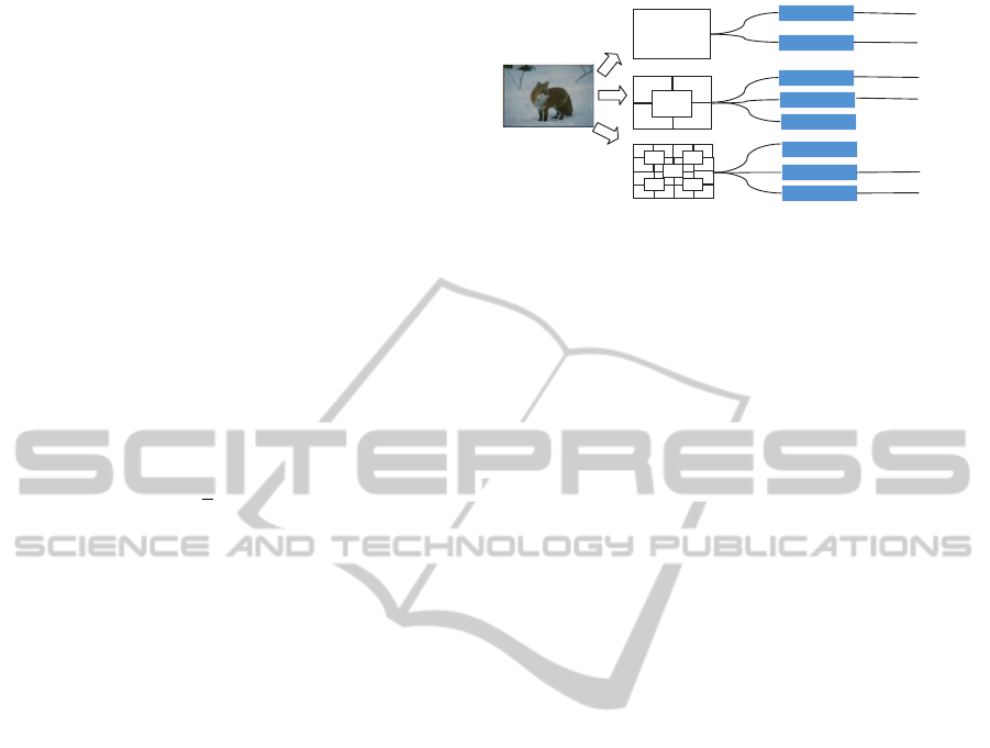
• Extracting Multi-level Features: we divide each
image in T different levels then perform M feature
extraction algorithms F
m
as in Figure 3. Here, we
X
1
X
2
X
3
X
4
…
…
X
M-1
X
M
F
1
F
2
F
3
F
4
…
…
F
M-1
F
M
Level 1
Level 2
Level 3
Figure 3: An image is divided into different levels of gran-
ularity. For a level, we perform one or more feature extrac-
tion methods. We then obtain M feature extraction methods.
can choose any suitable feature extraction such as
color, texture, shape description, gist, etc. for F
m
.
Let M (l) (l = 1,... , T) be indexes of feature ex-
tractions at level l, e.g. M (1) = 1,2;M (2) =
3,4,5 (Figure 3). From this notation, we have
∑
T
l=1
|M (l)| = M. Also, we can infer that all the
feature extraction algorithms at previous levels of
level l are indexed from 1 to min{M (l)} − 1.
• Cascade of Multi-instance Classifiers Over
Levels: given a label w, D
w
= {B
+
,B
−
} denotes
a training dataset where B
+
(B
−
) is the set of im-
ages with (without) w. Let Y be a vector of cor-
responding classes of images in D
w
, i.e. Y
n
= 1
if I
n
∈ B
+
and Y
n
= −1 otherwise. Let score be
the output (confidence) vector generated by ma-
chines (classifiers), where score
n
> 0 (or absolute
value of score
n
(< 0)) is the confidence of assign-
ing (not assigning) w to I
n
∈ D
w
. We denote h
m
the
weak classifier, which maps from feature space
X
m
of feature extraction algorithm F
m
to {−1,1}.
The confidence score posed by h
m
on the image
I is denoted by h
m
(F
m
(I)), that is we apply h
m
on feature vectors obtained by F
m
on I. Based
on these notations, CMLMI is presented in Algo-
rithm 1. Note that multi-instance learning turns
into single-instance learning at the coarsest level
when global feature vector is in use.
For global feature extractions at level l = 1, an im-
age has one instance (one feature vector), the problem
turns into normal supervised learning. We applied
SVM for this case. At finer level (l > 1), one image
has a set of instances, one corresponds to one subre-
gion. Due to weakly labeling, we do not know which
instance best represents the given label. The multiple-
instance version of SVM (MI-SVM) (see Section 4) is
used to address this ambiguity.
We update scores of images in D
w
at level l using
the following recursion:
score = H
l
= γ
l
∗ H
l−1
+
∑
m∈M (l)
α
m
∗ h
m
+ c
l
KDIR 2011 - International Conference on Knowledge Discovery and Information Retrieval
18

Algorithm 1: A Cascade of Multi-Level Multi-Instance Classifiers.
Input : A set D
w
= {B
+
,B
−
} of positive and negative examples for word w.
Output: A strong classifier H
w
for w
1 Initialize score
n
= 0, θ
i
= 1/|B
−
|, c = 0, and α
m
= 0 for n = 1,... , |B|, i = 1, ...,|B
−
|;, and m = 1, ...,M.
2 //Learning weak classifiers over T levels
3 for l ← 1 to T do
4 if l == 1 then
5 Learn classifiers h
m
using SVM from D
w
for all m ∈ M (l)
6 if l > 1 then
7 Sample a smaller set SB
−
from B
−
according to θ
8 Learn classifiers h
m
using MI-SVM from SD
w
= {B
+
,SB
−
} for all m ∈ M (l)
9 end
10 //Update score for all images in D
w
11 Set score
n
= γ
l
∗ score
n
+
∑
m∈M (l)
α
m
∗ h
m
(F
m
(I
n
)) + c
l
for n = 1, ...,|D
w
|
12 Find coefficients γ
l
> 0, α
m
and c
l
to minimize ||score−Y||
2
13 //Update coefficients of classifiers in previous levels
14 for m
′
= 1 to min{M (l)} − 1 do
15 α
m
′
= α
m
′
∗ γ
l
16 end
17 Update the overall threshold c = c∗ γ
l
+ c
l
18 Sort score in descending order, and let r
j
be the ranking position of I
j
∈ B
−
in sorted score
19 Update θ
j
← θ
j
∗ 1/r
j
for all j = 1, ...,|B
−
| and normalize θ so that
∑
j
θ = 1
20 end
21 Final robust classifier:
H
w
=
∑
M
m=1
α
m
∗ h
m
+ c
∑
M
m=1
α
m
+ c
Since we have the constraint that γ
l
> 0, the rank-
ing of images is based on previous ranking (H
l−1
) but
modified by the additional classifiers of current level
(the second term). The constant term c
l
is used as
the constant threshold for level l. We then find coeffi-
cients for classifiers of level l using linear regression
that is minimizing square error ||H −Y||
2
(lines from
10 to 11 in Algorithm 1). Here, scores for images in
D
w
are accumulated from level 1 to level l − 1 and
stored in score.
Unlike previous boosting methods, the sampling
distribution θ on B
−
is updated based on the rank-
ing positions of negative samples on the sorted score
instead of the score itself (line 18,19). As a result,
a negative example at higher rank will be weighted
more than negativeexamples at lower ranks. From the
experiments, we see that this ranking-based scheme is
better than score-based for unbalanced training set.
5.2 Detailed Analysis
This section presents theoretical analysis for our al-
gorithm, which focuses on the benefit of CMLMI in
training time and shows that our algorithm is suitable
to image annotation.
Based on cascading scheme, it is obvious that our
method requires less training time than learning all in-
dividual classifiers independently. The training time
of MI-SVM depends on |B
+
| + NR∗ |B
−
|, where NR
is the number of subregions per image. That NR is
larger on finer levels makes the domination of nega-
tive instances over positive ones even more serious.
Training MI-SVM in cascade with SB
w
(Line 7 in Al-
gorithm 1) is more efficient than training an indepen-
dent one with D
w
.
Not only having advantage in training time, but
also our method is suitable to image annotation and
able to reduce the ambiguity of weakly labeling.
When the coarse levels are in charge of detecting
related context of the given level, the finer levels
are able to focus on sample images of similar scene
to separate the object from the background, and re-
duce ambiguity caused by weakly labeling. Figure 4
demonstrates our idea. Here, circles still denote pos-
itive bags, in which we know positive instances are
available but do not know which ones, and triangles
denote negativebags, of which we have guarantee that
all instances are negative. The negative bag selected
here is the one with instances close to some other in-
stances of one positive bag (the red circle). The com-
CASCADE OF MULTI-LEVEL MULTI-INSTANCE CLASSIFIERS FOR IMAGE ANNOTATION
19
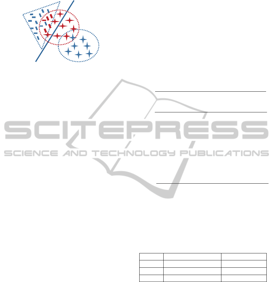
Figure 4: Negative bags that share common negative in-
stances with positive bags reduce ambiguity. Here the stars
denote unknown classes (either positive (+) or negative (-).
mon/similar instances correspond to subregions of the
shared/similar background of the two bags. Since we
have the knowledge that all instances of the negative
bag are negative, we can conclude that the instances
of the red circle, which are close to or even included
in the negative bag, are negative. Along with the sim-
ilarity among positive bags, which contain the same
object, this information helps to obtain better hyper-
plane to separate negative and positive instances. To
our best knowledge, this is one of the first attempts
that makes use of the similarity between negativebags
and positive bags to reduce ambiguity in MIL. Most
of previous approaches in MIL only made use of sim-
ilarity among positive bags to deal with the ambigu-
ity. For example, (Carneiro et al., 2007) only uses
positive bags to generalize a dominating distribution
over positive bags. (Maron and Lozano-P´erez, 1998)
finds regions in the instance space with instances from
many different positive bags and far away from in-
stances from negative bags. In (Yang et al., 2006;
Andrews et al., 2002), negative bags are sampled ran-
domly only to cope with the domination of negative
examples over positive examples without giving no-
tice to negative bags that share backgrounds with pos-
itive bags. Recently, (Deselaers and Ferrari, 2010)
also follows the idea that the significant portion of
positive instances will result in a reasonable classifier
performing better than by change. However, we ob-
serve that some negative instances also amount to sig-
nificant portion, which are the instances correspond-
ing to common backgrounds. This problem becomes
more serious when more and more labels are taken
into consideration like those in image annotation.
6 EXPERIMENTS
6.1 Corel5K Dataset
The Corel5k benchmark is obtained from Corel im-
age database and commonly used for image annota-
tion (Duygulu et al., 2002). It contains 5,000 images
and were pre-divided into a training set of 4,000 im-
ages, a validation set of 500 images, and a test set of
500 images. Each image is labeled with from 1 to 5
captions from a vocabulary of 374 distinct words.
6.2 Evaluation
Given a testing dataset, we can measure the effective-
ness of the algorithm. Regarding a label w, the typical
measures for retrieval are precision P
w
, recall R
w
:
P
w
=
Number of images correctly annotated with w
Number of images annotated with w
R
w
=
Number of images correctly annotated with w
Number of images manually annotated with w
We calculate P and R, which are means of P
w
and
R
w
over all labels. To balance the trace-off between
P and R, F
1
= 2 ∗ P ∗ R/(P + R) is usually used as
another measure for evaluation. In order to measure
retrieval performance, we also calculate the average
precision (AP) for one label w as follows:
AP
w
=
∑
N
r=1
P(r) × rel(r)
Number of images annotated manually with w
where r is a rank, N is the number of retrieved im-
ages, rel(r) is a binary function to check the word at
r is in the manual list of words or not, and P(r) is
the precision at r. Note that, the denominator of AP
is independent with N. Finally, mAP is obtained by
averaging APs over all labels of the testing dataset.
Table 1: Feature extractions & classifiers.
Level 1 F
1
: “gist” of scene SVM-GIST
- F
2
: color histogram SVM-color
Level 2 F
3
: color histogram MISVM-color
- F
4
: Gabor texture MISVM-texture
6.3 Experimental Settings
For the experiments, we performed a cascade of 4
classifiers with 2 levels. Here, we worked with only 2
levels because the images of Corel5K are all in small
size. Moreover, we would like to focus on the ba-
sic case to analyze the impact of global features on
reducing the weakly labeling problem. At the first
level, global features were extracted from the whole
image. We exploited Gist (Oliva and Torralba, 2001),
and color histogram in RGB color space with 16 chan-
nels. For each region in the second level, we also per-
formed color histogram extraction but with 8 channels
KDIR 2011 - International Conference on Knowledge Discovery and Information Retrieval
20
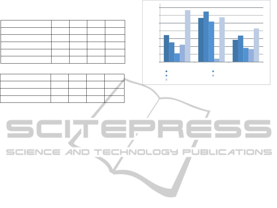
Table 2: CMLMI vs. various MIL methods.
(a) In comparison with other standalone MIL methods. Results of ASVM-
MIL and mi-SVM are reported in (Yang et al., 2006)
Method P R F1 mAP
ASVM-MIL 0.31 0.39 0.35 -
mi-SVM 0.28 0.35 0.31 -
MISVM-Color 0.13 0.55 0.21 0.19
MISVM-Texture 0.07 0.36 0.13 0.86
CMLMI 0.30 0.52 0.38 0.35
(b) In comparison with standalone SVM with global features
Method P R F1 mAP
SVM-Color 0.20 0.39 0.27 0.19
SVM-Gist 0.27 0.47 0.34 0.28
CMLMI 0.30 0.52 0.38 0.35
and texture extraction using Gabor filter as in (Maka-
dia et al., 2010). Summary of feature extraction meth-
ods and their relationship with levels are is given in
Table 1. The numbers of dimension in correspond-
ing feature spaces of algorithms F
1
,F
2
,F
3
, and F
4
are 960; 4096; 192; and 512 respectively.
We name classifiers trained on feature spaces
of F
1
,F
2
,F
3
, and F
4
as SVM-Gist, SVM-color,
MISVM-color, and MISVM-texture. Conventionally,
CMLMI is used to indicate the strong classifier H
w
learned according to Algorithm 1, in which classifiers
of level 2 (MISVM-color, and MISVM-texture) are
dependent of classifiers of level 1 (SVM-Gist, and
SVM-color). In the following, we refer to, for ex-
ample, MISVM-color (or standalone MISVM-color)
to indicate an independent classifier trained on D
w
,
and MISVM-color of CMLMI to imply the MISVM-
color learned in the cascade according to Algorithm
1. In the other words, MISVM-color of CMLMI is the
classifier trained on SD
w
sampled based on the results
of level 1 (SVM-Gist and SVM-color of CMLMI).
6.4 Experimental Results on 70 Most
Common Labels
Like (Yang et al., 2006), we selected 70 most common
labels from Corel5K dataset for experiments. The rea-
son is that labels with a small number of the positive
samples (for example: 5 10 positive samples) are not
efficient to train a classifier.
Table 2(a) shows that CMLMI outperforms other
MIL methods. As observable from the table, we
obtain improvements of 17.35% in F
1
measure and
16.14% in mAP compared to MISVM-color. In con-
trast to MISVM-texture, CMLMI significantly in-
creases F
1
measure by 25.64% and mAP by 26.71%.
Comparing to previous works, CMLMI obtains bet-
ter results than mi-SVM both in precision and recall,
which leads to a raise of 7.54% in F
1
measure. Also,
0.34
0.56
0.28
0.25
0.65
0.34
0.11
0.52
0.18
0.22
0.04
0.16
0.66
0.57
0.43
0.00
0.10
0.20
0.30
0.40
0.50
0.60
0.70
Tiger Horses Bear
Mean Average Precision
Standalone SVM-Gist Standalone SVM-Color
Standalone MISVM-Color Standalone MISVM-Texture
CMLMI
Figure 5: mAP of CMLMI in comparision with different
standalone methods.
CMLMI outperforms ASVM-MIL in recall while ob-
taining comparable precision (P of 0.30 with CMLMI,
and P of 0.31 with ASVM-MIL). This results in an
improvement 3.54% of our method over ASVM-MIL
in F
1
measure.
Table 2(b) compares CMLMI to SVM with global
features. We can see that CMLMI also obtain bet-
ter results in F
1
and mAP (F
1
of 0.38 and mAP of
0.35) compared with SVM-color (F
1
of 0.21 and mAP
of 0.20), and SVM-Gist (F
1
of 0.34, mAP of 0.27).
Among the standalone classifiers (SVM-color, SVM-
gist, MISVM-color, and MISVM-texture), SVM with
global features outperform MISVM with region-
based feature extractions. Interestingly, SVM-Gist
is even comparable to ASVM-MIL although image
segmentation, which is more expensive than global
feature, has been used in ASVM-MIL. However,
combining the classifiers in our cascading algorithm
yields the best results.
6.5 Experimental Results on Sample
Foreground Labels
We conducted carefully analysis for “tiger”, “horse”
and “bear” in Corel5K since the concepts correspond
to foreground objects which might benefit from finer
levels. Figure 5 shows mAP of standalone classi-
fiers and CMLMI for three labels. It can be seen
that individual feature types have different influences
on different labels. Except for Gist (F
1
) that shows
its importance for all three labels, global color his-
togram (F
2
) has more impact on annotating images
with “horses” and “bear” than with “tiger”. Texture
feature at level 2 (of MISVM-texture) performs better
than the other feature extraction methods only with
“tiger”. CMLMI significantly outperforms other stan-
dalone classifiers on “tiger” and “bear” while falls a
little on “horses” compared with SVM-color. Inter-
estingly, standalone MISVM-color is comparable to
CASCADE OF MULTI-LEVEL MULTI-INSTANCE CLASSIFIERS FOR IMAGE ANNOTATION
21
(a) Subregions selected by standalone MISVM-color
(b) Subregions selected by MISVM-color of CMLMI
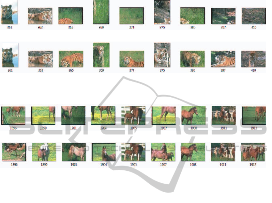
Figure 6: The subregions selected by standalone MISVM-color for label “tiger”, and the subregions selected by MISVM-color
of CMLMI from the corresponding images. Here, the numbers under each subregion indicate image IDs.
(a) Subregions selected by standalone MISVM-texture
(b) Subregions selected by MISVM-texture of CMLMI
Figure 7: The subregions selected by standalone MISVM-texture for label “horses” and the subregions (of corresponding
images) selected by MISVM-texture at the 2-nd level of CMLMI.
CMLMI for “horses”. In order to uncover the ques-
tion in the “horse” case, we conducted detailed anal-
ysis, and found that MISVM-color and SVM-color
captured grass fields in the background instead of
horses. Indeed, no subregion with the color of a horse
was considered in MISVM-color. Thus, the good
performance of standalone MISVM-color and SVM-
color owes to special feature of the Corel5K dataset in
which horses are on grass fields in most of pictures.
As previously mentioned, the negative examples
for finer levels are drawn based on the ambiguity
of coarser levels, which are able to detect the back-
ground better. By considering the negative examples
of similar background, we are able to add “negative
instances”, which usually appear with the real positive
instances of positive examples. As a result, there is
more chance for us to separate the ”positive instance”
from “negative instance” in positive examples. Figure
6 and Figure 7 show the examples of selecting posi-
tive instances from corresponding positive bags with
standalone MISVM and MISVM of CMLMI. We can
see from the figures that MISVM of CMLMI is able
to select more relevant subregions. For the case of
“tiger”, MISVM-color of CMLMI is given more in-
formation about background (grass, forest, stone, wa-
ter), it has successfully avoided selecting background-
related instances as positive ones.
7 CONCLUDING REMARKS
In this paper, we have presented an overview of im-
age annotation: its typical problems, feature extrac-
tion methods and typical methodologies. By analyz-
ing the main problems of image annotation, we pro-
posed a method based on cascading multi-level multi-
instance classifiers, which has main advantages as fol-
lows:
• Our cascade of MLMI classifiers is able to reduce
training time since we can remove some negative
examples, which are “easily” detected as negative
based on the scene, in finer levels.
• Multi-level feature extractions allow us to anno-
tate images with multiple resolutions. One exam-
ple is that a photo of tiger might be a close-up
photo or the photo of a tiger in its context. Multi-
level feature extractions bring more chance to cap-
ture all of this variety.
KDIR 2011 - International Conference on Knowledge Discovery and Information Retrieval
22

• We also show experimentally that it is able to re-
duce the ambiguity of “weakly labeling” in im-
age annotation, and separate the foreground ob-
jects from the scene in finer levels of the cascade.
The experiments show promising results of the
proposed method in comparison with several base-
lines on Corel5K. Experiments suggest that as long as
the finer levels can bring “newinformation”, they help
to obtain better detection of foreground objects. For
the future work, we would like to focus more on the
role of context in reducing the ambiguity of “weakly
labeling”.
REFERENCES
Akbas, E. and Vural, F. T. Y. (2007). Automatic image an-
notation by ensemble of visual descriptors. In IEEE
Conf. on CVPR, pages 1–8, Los Alamitos, CA, USA.
Andrews, S., Hofmann, T., and Tsochantaridis, I. (2002).
Multiple instance learning with generalized support
vector machines. In 18th AAAI National Conference
on Artificial intelligence, pages 943–944, Menlo Park,
CA, USA.
Barnard, K., Duygulu, P., Forsyth, D., Freitas, N. D., Blei,
D. M., K, J., Hofmann, T., Poggio, T., and Shawe-
taylor, J. (2003). Matching words and pictures. Jour-
nal of Machine Learning Research, 3:1107–1135.
Blei, D. M. and Jordan, M. I. (2003). Modeling annotated
data. In Proc. of the 26th ACM SIGIR, pages 127–134.
Carneiro, G., Chan, A. B., Moreno, P. J., and Vasconcelos,
N. (2007). Supervised learning of semantic classes for
image annotation and retrieval. IEEE Trans. PAMI,
29(3):394–410.
Deselaers, T. and Ferrari, V. (2010). A conditional random
field for multiple-instance learning. In Proc. of The
27th ICML, pages 287–294.
Deselaers, T., Keysers, D., and Ney, H. (2008). Features
for image retrieval: an experimental comparison. Inf.
Retr., 11:77–107.
Douze, M., J´egou, H., Sandhawalia, H., Amsaleg, L., and
Schmid, C. (2009). Evaluation of gist descriptors for
web-scale image search. In Proc. of the ACM CIVR,
pages 1–8, New York, NY, USA.
Duygulu, P., Barnard, K., de Freitas, J. F. G., and Forsyth,
D. A. (2002). Object recognition as machine transla-
tion: Learning a lexicon for a fixed image vocabulary.
In Proc. of the 7th ECCV, pages 97–112, London, UK.
Springer-Verlag.
Feng, S. L., Manmatha, R., and Lavrenko, V. (2004). Mul-
tiple bernoulli relevance models for image and video
annotation. In Proc. of the 2004 CVPR.
Hofmann, T. (1999). Probabilistic latent semantic indexing.
In Proc. of the 22nd ACM SIGIR, pages 50–57, New
York, NY, USA.
J´egou, H., Douze, M., and Schmid, C. (2010). Improving
bag-of-features for large scale image search. Int. J.
Comput. Vision, 87(3):316–336.
Jeon, J., Lavrenko, V., and Manmatha, R. (2003). Au-
tomatic image annotation and retrieval using cross-
media relevance models. In Proc. of the 26th int. ACM
SIGIR, pages 119–126.
Jeon, J., Lavrenko, V., and Manmatha, R. (2004). Auto-
matic image annotation of news images with large vo-
cabularies and low quality training data. In Proc. of
ACM Multimedia.
Kennedy, L. S. and Chang, S.-F. (2007). A reranking ap-
proach for context-based concept fusion in video in-
dexing and retrieval. In Proc. of the 6th ACM int. on
CIVR, pages 333–340, New York, NY, USA. ACM.
Lavrenko, V., Manmatha, R., and Jeon, J. (2003). A model
for learning the semantics of pictures. In Advances
in Neural Information Processing Systems (NIPS’03).
MIT Press.
Lazebnix, S., Schmid, C., and Ponce, J. (2009). Object Cat-
egorization: Computer & Human Vision Perspectives,
chapter Spatial Pyramid Matching. Cambridge Uni-
versity Press.
Makadia, A., Pavlovic, V., and Kumar, S. (2010). Base-
lines for image annotation. Int. J. Comput. Vision,
90(1):88–105.
Maron, O. and Lozano-P´erez, T. (1998). A framework for
multiple-instance learning. In Proc. of the Conf. on
Advances in Neural Information Processing Systems,
NIPS ’97, pages 570–576, Cambridge, MA, USA.
MIT Press.
Monay, F. and Gatica-Perez, D. (2007). Modeling semantic
aspects for cross-media image indexing. IEEE Trans.
Pattern Anal. Mach. Intell., 29(10):1802–1817.
Nguyen, C.-T., Kaothanthong, N., Phan, X.-H., and
Tokuyama, T. (2010). A feature-word-topic model for
image annotation. In Proc. of the 19th ACM CIKM,
pages 1481–1484.
Oliva, A. and Torralba, A. (2001). Modeling the shape of
the scene: A holistic representation of the spatial en-
velope. Int. J. of Comput. Vision, 42:145–175.
Sch¨olkopf, B., Burges, C. J. C., and Smola, A. J., editors
(1999). Advances in kernel methods: support vector
learning. MIT Press, Cambridge, MA, USA.
Szummer, M. and Picard, R. W. (1998). Indoor-outdoor
image classification. In Proc. of the 1998 Int. Work-
shop on Content-Based Access of Image and Video
Databases, page 42, Washington, DC, USA.
Torralba, A., Murphy, K. P., and Freeman, W. T. (2010).
Using the forest to see the trees: exploiting context
for visual object detection and localization. Commun.
ACM, 53(3):107–114.
Viola, P. and Jones, M. (2001). Rapid object detection using
a boosted cascade of simple features. In Proc. of IEEE
CVPR, volume 1, pages I–511 – I–518 vol.1.
Yang, C., Dong, M., and Hua, J. (2006). Region-based
image annotation using asymmetrical support vector
machine-based multiple-instance learning. In Proc. of
the 2006 IEEE CVPR, pages 2057–2063, Washington,
DC, USA.
CASCADE OF MULTI-LEVEL MULTI-INSTANCE CLASSIFIERS FOR IMAGE ANNOTATION
23
