
HASHMAX: A NEW METHOD FOR MINING MAXIMAL
FREQUENT ITEMSETS
Natalia Vanetik and Ehud Gudes
Deutsche Telecom Laboratories and CS department, Ben Gurion University, Beer-Sheva, Israel
Keywords:
Maximal frequent itemset mining.
Abstract:
Mining maximal frequent itemsets is a fundamental problem in many data mining applications, especially in
the case of dense data when the search space is exponential. We propose a top-down algorithm that employs
hashing techniques, named HashMax, in order to generate maximal frequent itemsets efficiently. An empirical
evaluation of our algorithm in comparison with the state-of-the-art maximal frequent itemset generation algo-
rithm Genmax shows the advantage of HashMax in the case of dense datasets with a large amount of maximal
frequent itemsets.
1 INTRODUCTION
The task of finding frequent itemsets in transactional
databases is an essential problem and a first step in
many data mining applications, such as finding asso-
ciation rules, relational data modeling etc. Because
of the time and space complexity required to find all
frequent itemsets in a database, sub-problems of find-
ing only closed frequent itemsets (the itemsets that
are not contained in a superset with the same sup-
port) or maximal frequent itemsets (the itemsets that
are not a subset of other frequent itemsets) have been
defined and studied. The set of maximal frequent
itemsets is orders of magnitude smaller than the set
of closed frequent itemsets, which itself is orders of
magnitude smaller than the set of frequent itemsets.
When the frequent patterns are long and their num-
ber is significant, sets of frequent itemsets and even
closed frequent itemsets become very large and most
traditional methods count too many itemsets to be fea-
sible. For the case of dense datasets, both traditional
frequent itemset search and closed itemset search be-
come inefficient due to the very large number of pat-
terns found. Therefore, several algorithms for max-
imal frequent itemset mining have been suggested.
The Pincer Search algorithm (Lin and Kedem, 1998)
uses both the top-down and bottom-up approaches to
frequent itemset mining. The MaxEclat and Max-
Clique algorithms, proposed in (Zaki et al., 1997),
identify maximal frequent itemsets by attempting to
look ahead and identify long frequent itemsets in or-
der to prune the search space efficiently. The
MaxMiner algorithm for mining maximal frequent
itemsets, presented in (Bayardo, 1998), is based on
a breadth-first traversal approach. The DepthProject
algorithm, presented in (Agarwal et al., 2000), finds
long itemsets using a depth-first search of a lexico-
graphic tree of itemsets, and uses a counting method
based on transaction projections along its branches.
The Mafia algorithm (Burdick et al., 2001) uses elab-
orate pruning strategies to get rid of non-maximal
sets, namely subset inclusion, TID set inclusion and
look-ahead pruning. The Fpgrowth algorithm of (Han
et al., 2000) and (Hu et al., 2008) uses a pattern
growth approach to frequent itemset and maximal fre-
quent set generation, completely eliminating the need
for candidate generation. The Genmax algorithm pro-
posed in (Gouda and Zaki, 2005) finds all maximal
frequent itemsets by efficiently enumerating the item-
sets with the help of a backtracking search. Genmax
is currently considered to be the state-of-the-art al-
gorithm and has been shown to outperform the Mafia
algorithm (Burdick et al., 2001) and the MaxMiner al-
gorithm (Bayardo, 1998), which in turn outperforms
the Pincer Search algorithm (Lin and Kedem, 1998).
In this paper, we propose a new HashMax algo-
rithm that uses hashing and a top-down approach for
maximal frequent itemset generation. The algorithm
starts with a set of candidates, where each candi-
date corresponds to a (pruned) set of items in each
transaction, and continues downwards until a maxi-
mal frequent itemset is discovered. Combined with
efficient pruning and subset generation, this approach
allows us to efficiently find maximal frequent item-
140
Vanetik N. and Gudes E..
HASHMAX: A NEW METHOD FOR MINING MAXIMAL FREQUENT ITEMSETS.
DOI: 10.5220/0003628101320137
In Proceedings of the International Conference on Knowledge Discovery and Information Retrieval (KDIR-2011), pages 132-137
ISBN: 978-989-8425-79-9
Copyright
c
2011 SCITEPRESS (Science and Technology Publications, Lda.)

sets in dense datasets, beginning with the largest ones.
The HashMax algorithm is designed specially for the
dense dataset and low support case; however, on very
sparse dataset our algorithm is also able finish quickly
by using initial dataset pruning. We evaluated Hash-
Max by comparing its performance to Genmax, a cur-
rent state-of-the art algorithm for mining maximal fre-
quent itemsets on several datasets of varying sizes and
density. In the rest of the paper, we proceed in the
following order: section 2 gives basic definitions and
outlines the algorithm, section 3 describes the algo-
rithm in detail, and section 4 deals with implementa-
tion issues and experimental evaluation.
2 FINDING MAXIMAL
FREQUENT ITEMSETS
We are given a transaction database D of size |D|,
whose tuples t = (item
1
,...,item
n
t
) consist of items
item
1
,...,item
n
t
, and the number of items can vary
from tuple to tuple. We are also given a user-defined
real valued support threshold S ∈ [0,1]. An itemset is
a set of items such that every item appears in some
transaction of D. The size of an itemset is the num-
ber of items in it. The support of an itemset I is
supp(I) :=
count(I)
|D|
, where count(I) denotes the num-
ber of transactions in D containing all the items of I.
Itemset I is frequent if supp(I) ≥ S. Itemset I is called
maximal frequent if it is a frequent itemset and it is
not contained (as a set) in any other frequent itemset.
The objective of a maximal frequent itemset min-
ing algorithm is to find a collection F of all maximal
frequent itemsets. F is a union of F
1
,...,F
max
, where
each F
i
contains all maximal frequent itemsets of size
i. Here and further, we denote by C
i
a set of item-
sets of size i that are thought to have a potential to be
maximal frequent during the search performed by a
maximal frequent itemset mining algorithm. The set
C
i
is called a candidate set. Each C
i
is superset of F
i
.
In this paper, we propose the HashMax algorithm
for finding maximal frequent itemsets in a top-down
fashion, while using hashing as a method for com-
puting the itemsets’ support. We start with maximal-
sized itemsets and proceed to smaller itemsets. As a
result, when an itemset is declared frequent, it is also
maximal since smaller itemsets have not been gener-
ated yet. Special attention must be given to subsets
of already discovered maximal frequent itemsets, as
those subsets are frequent but not maximal. The al-
gorithm uses a single database scan to build initial
structures, and is iterative. Maximal itemsets of size
(max − i + 1) are built at iteration i, where max is
the size of the largest maximal frequent itemset in the
database. The main steps of our algorithm are:
1. Initial Scan Phase. scan the database and gener-
ate candidate set C
max
, frequent set F
1
containing
frequent itemsets of size 1, and coverage set F
cover
containing a space-saving representation of F
2
.
2. F
1
Pruning. remove from F
1
all items whose
count is is |D| as these items are members of ev-
ery maximal frequent itemset and need not to be
taken into consideration.
3. Main Pruning Phase. go over every candidate
itemset I ∈ C
max
and delete from I all the items
that do not appear in pruned F
1
. Afterward,
remove from F
cover
all entries corresponding to
items not in F
1
.
4. Generation Phase. performed for every non-
empty candidate set C
i
. Go over each candi-
date itemset I ∈ C
max
add I to frequent set F
|I|
if
supp(I) ≥ S. Otherwise, if I is not contained in an
already generated frequent itemset, add subsets of
I of size |I| − 1 to candidate set C
|I|−1
.
5. Stop Criteria. stop when current candidate item-
set C
i
is empty.
In order to generate candidate itemsets, we need three
main data structures. First is the candidate set hash
table, denoted by C
i
. Each itemset I is stored at place
p(I) inC
i
. A pass over the hash tableC
i
generates can-
didate itemsets for the table C
i−1
and frequent item-
sets for the set F
i
. The second data structure we need
is the itemset I itself, that must keep a list of its items
and the source list, which is our third main data struc-
ture. The source list is a structure that is built gradu-
ally during as the algorithm is iterated. For an item-
set I ∈ C
max
, its source list I.source contains the hash
value p(I) of I in the hash table C
max
and the number
of database tuples containing I. This value is com-
puted during the initial database scan. For an itemset
I ∈ C
i
, i < max, I.source is the union of source lists
as sets for all candidate itemsets J ∈ C
max
containing
I as a subset. The candidate list of I replaces the need
to track transaction IDs by tracking bucket IDs in the
hash tableC
max
, since the number of buckets is in gen-
eral much smaller than the number of transactions.
3 THE HASHMAX ALGORITHM
3.1 Initial Scan and F
1
Creation and
Pruning
During the initial scan, described in Algorithm 1, we
build two sets: the first frequent set, denoted F
1
, and
the last candidate set in a form of a hash table, denoted
HASHMAX: A NEW METHOD FOR MINING MAXIMAL FREQUENT ITEMSETS
141

Algorithm 1: Initial scan phase.
Input: database D, support S
Output: frequent sets F
1
and F
cover
, candidate set
C
max
, database size |D|
1: F
1
:=
/
0, C
max
:=
/
0, |D| := 0
2: for all tuples t = (t
1
,...,t
n
t
) ∈ D do
3: sort t so that t
1
≤ ... ≤ t
n
t
;
4: p := hash(t
1
,...,t
n
t
);
5: C
max
[p].itemset:=t;
6: C
max
[p].count + +;
7: for i = 1 to n
t
do
8: q := hash(t
i
); F
1
[q].count + +;
9: for j = i+ 1 to n
t
do
10: r := hash(t
j
);
11: F
cover
[q][r].count + +;
12: end for
13: end for
14: |D| + +;
15: end for
16: // F
1
pruning
17: for all i s.t. F
1
[i].count < S|D|
or F
1
[i].count == |D| do
18: F
1
[i] :=
/
0;
19: end for
20: for all i s.t. F
1
[i] ==
/
0 do F
cover
[i][ j] :=
/
0;
Algorithm 2: Main pruning phase.
Input: frequent sets F
1
and F
cover
,
candidate set C
max
,
database size |D|,
support S.
Output: maximal size max of candidate itemsets,
set of candidate itemsets C
max
,
1: max := 0;
2: for all itemsets
t = (item
1
,...,item
n
t
) ∈ C
max
do
3: for j = 0 to n
t
do
4: let p := hash(item
i
);
5: if F
1
[p].count =
/
0 then
6: t := t \ {item
i
};
7: end if
8: end for
9: if max < |t| then
10: max := |t|;
11: end if
12: end for
13: for all itemsets t ∈ C
max
do
14: if |t| < max then
15: move t to C
|t|
;
16: end if
17: end for
maxC
maxC
maxC
F
1
remove
infrequent
or too
frequent
items
frequent
bid=2: 1,4,6,7
bid=3: 1,2,6,7
bid=4: 1,5,6,7
frequent
itemsets
remove
bid=3: 2,6,7 count=1
bid=2: 4,6,7 count=3
bid=5: 6,7 count=1
bid=1: 1,2,3,4
bid=2: 1,4,6,7
bid=3: 1,2,6,7
bid=4: 1,5,6,7
{2},{3},{4}.{6},{7}
Figure 1: Pruning candidate set C
max
.
C
max
, where max is the size of the largest itemset in
the scanned relations. We assume that a good hash
function is chosen for this purpose and collision han-
dling is a part of hash table implementation. F
1
con-
tains all items in D with their respective counts, F
cover
contains all pairs of items in D with their counts, and
C
max
contains all itemsets that appear in D as trans-
actions. All itemset counts are assumed to be 0 at
the start. Since the initial scan allows us to determine
the database size |D|, a simple pass over F
1
and F
cover
using values |D| and S (user-defined support value)
prunes out all non-frequent itemsets of size ≤ 2. Dur-
ing the pruning phase of Algorithm 2, we leave only
frequent items in each itemset generated so far, i.e.
items contained in F
1
in the candidate set C
max
. Some
of the candidate itemsets will shrink in size as a result
of the pruning. Figure 1 shows the pruning process
of a sample itemset C
max
. The first pruning step is re-
moving itemsets that are already frequent and report-
ing them to the user. In this example, itemset 1,2,3,4
is frequent. The second step of pruning consists of re-
moving from every transaction 1-itemsets that do not
appear in F
1
. If a 1-itemset is too frequent ({1} in our
example), it is excluded from the mining process but
later reported as part of every frequent itemset.
3.2 Candidate Generation
Generating itemsets for the next iteration is a task that
needs to be approached with care. The purpose of the
Subsets() function is not to generate an itemset with
the same source list twice. Let t = (item
1
,...,item
n
)
be a non-frequent candidate itemset. We observe the
following.
• Every subset t
¬i
:= t \ item
i
is a candidate itemset
of size |t| − 1.
KDIR 2011 - International Conference on Knowledge Discovery and Information Retrieval
142

• A subset t
′
of t
¬i
of size |t| − 2 is also a subset of
t
¬ j
if it does not contain item
j
.
We introduce set parameter t
¬i
.mandatory of the
itemset t
¬i
, whose value determines which subsets of
t
¬i
are not generated by other subset t
¬ j
. An order
t
¬1
< ... < t
¬n
allows us to make sure that no sub-
set of size |t| − 2 is missed – we set t
¬i
.mandatory =
{item
1
,...,item
i−1
}. Indeed, if an itemset t
′
⊂ t
¬i
has
size |t| − 2 and is not contained none of t
¬1
,...,t
¬i−1
then it contains all the items item
1
,...,item
i−1
. Thus,
no subset is missed and no subset is generated twice.
The procedure for sub-itemset generation is shown in
Algorithm 4.
3.3 Cleaning Itemsets
Once a candidate itemset t has been generated and
t.mandatory parameter has been set, we can use the
frequent 2-itemset data stored in F
cover
in order to
reduce the size of t (the cleaning process). The
items in t.mandatory need to remain in t in order
to allow further subset generation. Therefore, a pair
item
1
,item
2
∈ t.mandatory must be contained in a
frequent 2-itemset in order for t to contain a maxi-
mal frequent itemset of size ≥ 3. Function Clean()
in Algorithm 5 performs the task of removing all
items from t that are not paired together with items
in t.mandatory in a frequent 2-itemset.
Algorithm 3: HashMax algorithm.
Input: candidate set C
max
, support S, database size
|D|, maximal itemset size max, F
cover
Output: maximal frequent sets F
max
,...,F
3
1: i := max
2: while C
i
is not empty and i ≥ 3 do
3: for all itemsets t = (item
1
,...,item
i
) ∈ C
i
do
4: if count(t) ≥ S|D| then
5: F
i
:= F
i
∪ {t};
6: else
7: subsets(t) :=Subsets(t);
8: for all itemsets I ∈ subsets(t) do
9: Clean(I, F
cover
);
10: if |I| > 2 and I /∈ ∪F
i
then
11: p := hash(I);
12: add I.sourcelist to C
|I|
[p].sourcelist;
13: end if
14: end for
15: end if
16: end for
17: i− −;
18: end while
19: return ∪F
i
;
Algorithm 4: Subsets.
Input: itemset t = (item
1
,...,item
n
)
Output: subsets of t of size n − 1 with mandatory
parameter set.
1: subsets(t) :=
/
0;
2: for i = 1 to n do
3: t
¬i
.mandatory := {item
j
| j < i};
4: subsets(t) := subsets(t) ∪ {t
¬i
};
5: end for
6: return subsets(t);
Algorithm 5: Clean().
Input: itemset t = (item
1
,...,item
n
), F
cover
, database
size |D|, support S
Output: reduced itemset t
1: for all item
1
∈ t \ t.mandatory, item
2
∈
t.mandatory do
2: if F
cover
[hash(item
1
)][hash(item
2
)] =
/
0 then
3: t := t \ {item
1
};
4: end if
5: end for
6: return t;
Figure 2 illustrates the process of an itemset clean-
ing.
3.4 The Mining Phase
The mining phase of our algorithm consists of scan-
ning the current candidate set C
i
, extracting frequent
itemset into set F
i
and creating candidates for the set
C
i−1
from the non-frequent itemsets of C
i
. Subsets
of frequent itemsets are frequent but not maximal and
therefore are not used for further mining.
Main cycle in lines 2 − 19 of Algorithm 3 iter-
ates over the candidate itemset size. At iteration i,
lines 4 − 5 of the algorithm generate frequent item-
sets of size i. These itemsets are maximal because
line 10 makes sure that no new candidate is contained
in already generated frequent itemsets. Lines 7− 8 of
Algorithm 3 generate candidate itemsets of size i− 1
from a non-frequent itemset of size i. After clean-
ing the candidate in line 9, the newly generated can-
didate itemset is placed in the appropriate hash table
representing the corresponding candidate set. Since
a single candidate of size i− 1 may arise as a subset
of more than one non-frequent candidate itemset of
size i, the source list of a new candidate must be the
union of source lists of all candidate itemsets contain-
ing it as a subset (lines 12− 13). The time complexity
of the problem of finding all maximal frequent item-
sets is known to lie in Pspace and is well studied (see,
HASHMAX: A NEW METHOD FOR MINING MAXIMAL FREQUENT ITEMSETS
143
F
cover
items=1,2
items=2,3
items=1,3
process
The cleaning
1,2,3,4
mandatory={}
2,3,4
1,2,4 1,2,3 1,3,4
mandatory={} mandatory={1} mandatory={1,2} mandatory={1,2,3}
clean candidates
2,3 1,3 1,2 1,2,3
Figure 2: Cleaning itemsets with the help of F
cover
.
e.g. (Yang, 2004)). The precise complexity of any al-
gorithm that finds maximal frequent itemsets entirely
depends on the distribution of the data in a specific
dataset. The space complexity of HashMax is con-
stant for each run and is at most O(n
2
), where n is
the number of transactions. If a bitmap source list
representation is used, the space complexity of Hash-
Max algorithm decreases to O(nlogn). At iteration k,
the total space used by the algorithm is bounded by
n
2
avg(count(t)−1)
where the average is taken over all fre-
quent k-itemsets t, and by
nlogn
avg(count(t)−1)
for the bitmap
representation, where the average is taken over all fre-
quent k-itemsets.
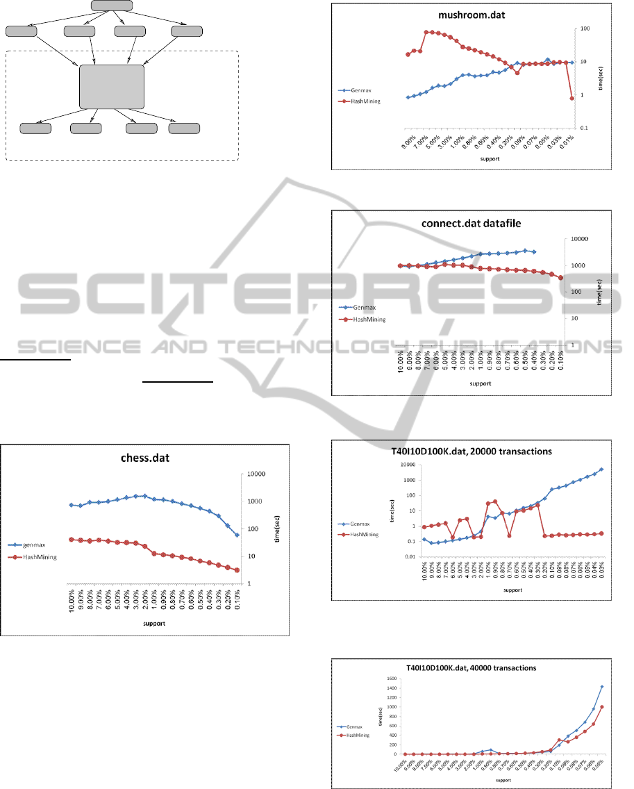
Figure 3: Comparison on the chess.dat database.
4 EXPERIMENTAL EVALUATION
The HashMax algorithm was implemented in Java
and it was tested on a machine with Intel Xeon
2.60GHz CPU and 3Gb of main memory running
Linux OS. We have compared HashMax to the Gen-
max algorithm ((Gouda and Zaki, 2005)), using ef-
ficient implementation available at (Genmax, 2011).
In all charts, the X axis denotes support in % while
the Y axis denotes the time that it took the algorithm
to produce all maximal frequent itemsets for a given
Figure 4: Comparison on the mushroom.dat database.
Figure 5: Comparison on the connect.dat database.
Figure 6: Comparison on a sparse database with 20000
transactions.
Figure 7: Comparison on a sparse database with 40000
transactions.
KDIR 2011 - International Conference on Knowledge Discovery and Information Retrieval
144
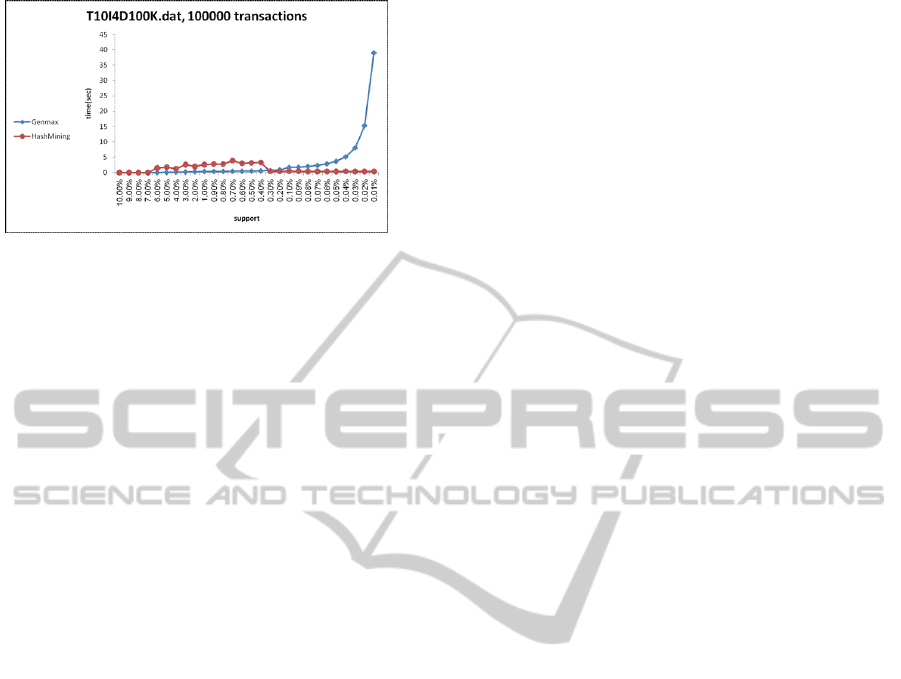
Figure 8: Comparison on a sparse database with 100000
transactions.
support value, in seconds. In Figures 3-6 we used log-
scale for the Y axis in order to show the difference in
small running times better.
We tested both algorithms on several datasets with
different sizes and characteristics from the UCI ma-
chine learning repository (the datasets are available
at (UCI, 2011)). The chess.dat file contains 3196
transactions and is a dense dataset (a dense dataset
is a dataset that contains transactions with many com-
mon items). The number of maximal frequent item-
sets in chess.dat varies from tens for very high sup-
port values to over ten thousand for lower support
values. The mushroom.dat file contains 8124 trans-
actions and is a relatively sparse dataset. It con-
tains thousands of maximal frequent itemsets for low
support values. The connect.dat file contains 67557
transactions and represents a dense dataset (for low
support values, it contains up to 17000 maximal fre-
quent itemsets). The number of items in each trans-
action is large and is constant for chess.dat, mush-
room.dat and connect.dat. Datasets T10I4D100K.dat
and T40I10D100K.dat have variable transaction size
and are very sparse. These datasets contain no maxi-
mal frequent itemsets of size larger than 2 for higher
support values and several thousands maximal fre-
quent itemsets for very low support values. Fig-
ure 3 shows a comparison both algorithms on the
chess.dat dataset. We see that due to the density of
this dataset HashMax always shows substantially bet-
ter times than Genmax. Figure 4 shows a comparison
of both algorithms on the mushroom.dat dataset. Be-
cause this dataset is sparse, HashMax gains an advan-
tage over Genmax for lower support values. Figure
5 shows a comparison both algorithms on the con-
nect.dat dataset. As this dataset is quite dense, Hash-
Max consistently shows better times than Genmax.
Figures 6 and 7 show a comparison of the two al-
gorithms on parts of T40I10D100K.dat of different
sizes (20000 transactions and 40000 transactions re-
spectively). Since the original dataset is very sparse,
HashMax shows better results for lower support val-
ues. Figure 8 shows a comparison of the two algo-
rithms on large (1000000 transactions) sparse dataset
T10I4D100K.dat. The algorithms show similar times
for medium support values, but HashMax times are
much better for low support values. In conclusion, we
have found that HashMax outperforms Genmax for
dense datasets (i.e. when the total number of maximal
frequent itemsets is significant) throughout and for
low support values when tested on sparse datasets).
For support values in the range of 0-0.1% the differ-
ence in running time was quite noticeable.
ACKNOWLEDGEMENTS
Authors thank the Lynn and William Fraenkel Cen-
ter for Computer Science for partially supporting this
work.
REFERENCES
Agarwal, R., Aggarwal, C., and Prasad, V. (2000). Depth
first generation of long patterns. In ACM SIGKDD
Conf.
Bayardo, R. J. (1998). Efficiently mining long patterns from
databases. In ACM SIGMOD Conf. on Management of
Data, pages 85–93.
Burdick, D., Calimlim, M., and Gehrke, J. (2001). Mafia, a
maximal frequent itemset algorithm for transactional
databases. In IEEE Intl. Conf. on Data Engineering,
pages 443–452.
Genmax (2011). Genmax implementa-
tion. http://www.cs.rpi.edu/ zaki/www-
new/pmwiki.php/Software.
Gouda, K. and Zaki, M. J. (2005). Genmax: An efficient
algorithm for mining maximal frequent itemsets. Data
Mining and Knowledge Discovery 11(3), pages 223–
242.
Han, J., Pei, J., and Yin, Y. (2000). Mining frequent patterns
without candidate generation. In ACM SIGMOD Conf.
on Management of Data, pages 1–12.
Hu, T., Sung, S. Y., Xiong, H., and Fu, Q. (2008). Discov-
ery of maximum length frequent itemsets. In Inf. Sci.
178(1), pages 69–87.
Lin, D.-I. and Kedem, Z. M. (1998). Pincer search: A new
algorithm for discovering the maximum frequent set.
In EDBT, pages 105–119.
UCI (2011). Uci machine learning data repository.
http://archive.ics.uci.edu/ml/index.html.
Yang, G. (2004). The complexity of mining maximal fre-
quent itemsets and maximal frequent patterns. In
KDD, pages 344–353.
Zaki, M. J., Parthasarathy, S., Ogihara, M., and Li, W.
(1997). New algorithms for fast discovery of associa-
tion rules. In Third Int 1 Conf. on Knowledge Discov-
ery in Databases and Data Mining, pages 283–286.
HASHMAX: A NEW METHOD FOR MINING MAXIMAL FREQUENT ITEMSETS
145
