A HYBRID APPROACH TO LOCALLY OPTIMIZED

INTERPRETABLE PARTITIONS OF FUZZY NEURAL MODELS

Wanqing Zhao

, Kang Li

, George W. Irwin

and Qun Niu

Intelligent Systems and Control, Queen’s University Belfast, Stranmillis Road, Belfast, U.K.

School of Mechatronical Engineering and Automation, Shanghai University, Shanghai, China

Keywords:

Fuzzy neural systems, Interpretable model, Differential evolution, Weighted fast recursive algorithm, ANFIS.

Abstract:

Many learning methods have been proposed for Takagi-Sugeno-Kang fuzzy neural modelling. However, de-

spite achieving good global performance, the local models obtained often exhibit eccentric behaviour which

is hard to interpret. The problem here is to ﬁnd a set of input space partitions and, hence, to identify the corre-

sponding local models which can be easily understood in terms of system behaviour. A new hybrid approach

for the construction of a locally optimized, functional-link-based fuzzy neural model is proposed in this paper.

Unlike the usual linear polynomial models used for the rule consequent, the functional link artiﬁcial neural

network (FLANN) is employed here to achieve a nonlinear mapping from the original model input space.

Our hybrid learning method employs a modiﬁed differential evolution method to give the best fuzzy partitions

along with the weighted fast recursive algorithm for the identiﬁcation of each local FLANN. Results from a

motorcycle crash dataset are included to illustrate the interpretability of the resultant model structure and the

efﬁciency of the new learning technique.

1 INTRODUCTION

Takagi-Sugeno-Kang (TSK) fuzzy neural systems

have been widely applied to the modelling of nonlin-

ear dynamic systems from noisy datasets. In fact, a

TSK fuzzy model can be viewed as a number of lo-

cal models valid in different input spaces. However,

due to the linear polynomial form of the rule conse-

quent, this representation may not capture fully all the

information contained in the original input space. A

functional-link-based neural fuzzy network, consist-

ing of nonlinear combinations of the model inputs has

therefore been proposed for the rule consequent (Lin

et al., 2009).

The most important issue for nonlinear modelling

is to optimize the fuzzy neural system parameters us-

ing the given data. To deal with possible local min-

ima, heuristic algorithms can either be directly ap-

plied, or else integrated with more conventionalmeth-

ods to enhance the training accuracy. For example

the random optimization approach has been success-

fully used to update the premise parameters (Cheng,

2009). Given sufﬁcient rules and training data, there

are many techniques available for producing an accu-

rate TSK fuzzy model. However, the interpretability

of the local models obtained cannot always be guar-

anteed.

The goal of this paper is to construct a locally

optimized fuzzy neural model, consisting of a set of

fully-interpretable local models. Unlike (Lin et al.,

2009), the parameters to be learned are divided into

two subsets, corresponding to the premise and con-

sequent parts of the model. A simple modiﬁcation

to differential evolution (DE) is described and then

utilized to optimize the nonlinear parameters in the

rule premises. A weighted version of the fast recur-

sive algorithm (FRA) (Li et al., 2005) is also derived

for determining the structure and identifying the lin-

ear parameters locally in the rule consequents. An

application study and comparison with ANFIS illus-

trated the interpretability of the resultant model struc-

ture and the efﬁciency of the new learning technique.

2 FUNCTIONAL-LINK-BASED

FUZZY NEURAL SYSTEMS

Functional-link-based fuzzy neural systems are repre-

sented by the following:

(t) = A

i,1

AND

(t) = A

i,2

AND

...

AND

(t) = A

i,n

THEN

ˆy

(t) = f

(t);θ

)

(1)

461

Zhao W., Li K., W. Irwin G. and Niu Q..

A HYBRID APPROACH TO LOCALLY OPTIMIZED INTERPRETABLE PARTITIONS OF FUZZY NEURAL MODELS.

DOI: 10.5220/0003626304610465

In Proceedings of the International Conference on Evolutionary Computation Theory and Applications (FCTA-2011), pages 461-465

ISBN: 978-989-8425-83-6

 2011 SCITEPRESS (Science and Technology Publications, Lda.)

where i is the rule index, X(t) = [x

(t),...,x

(t)]

∈

ℜ

represents the n model inputs, A

i, j

is the fuzzy set

associated with the ith rule corresponding to the input

, ˆy

(t) is the local model output realized using the

output of a functional link artiﬁcial neural network

(·), Z

(t) = [z

i,1

(t),...,z

i,q

(t)]

∈ ℜ

deﬁnes the q

most signiﬁcant basis functions of the input variables

selected for the ith output of the FLANN, and θ

is the

corresponding coefﬁcient vector.

In a FLANN, the input vector X(t) is functionally

enhanced by a set of linearly independent functions

chosen from an orthonormal basis set, to give the out-

put s

(t):

(t) =

∑

j=1

i, j

(X(t)) (2)

where q denotes the total number of functional ex-

pansions for all inputs, θ

i, j

is the weight parameter

relating to the ith output of the FLANN and p

repre-

sents the jth basis function. As with (Lin et al., 2009),

trigonometric expansions are used for the expanders.

Now the ith output of FLANN is taken as the conse-

quent part for the ith rule. To give a compact local

model, and to enhance the understandability, a subset

of the most signiﬁcant combination of terms se-

lected from (2) form the ith rule consequent. Thus

(t);θ

) =

∑

j=1

i, j

(t); j = 1,...,q

(3)

Here θ

= [θ

i,1

,...,θ

i,q

]

∈ ℜ

are the coefﬁ-

cients associated with the ith output of the FLANN.

For N data samples, z

i, j

= [z

i, j

(1),...,z

i, j

(N)]

∈

ℜ

and p

(X) = [p

(X(1)),..., p

(X(N))]

∈ ℜ

then Z

= [z

i,1

,...,z

i,q

] will be a subset of P =

(X),...,p

(X)].

Assuming Gaussian membership functions are

used in the fuzzy sets, the ﬁring strength of the ith

fuzzy rule can be computed from the T-norm:

(X(t);w

) =

∏

j=1

exp

(

−



(t) − c

i, j



)

(4)

where c

i, j

and σ

i, j

denote the centre and stan-

dard deviation of A

i, j

, w

= [c

,σ

]

∈ ℜ

, c

i,1

,...,c

i,n

]

∈ ℜ

, and σ

= [σ

i,1

,...,σ

i,n

]

∈ ℜ

The normalized ﬁring strength of the ith rule which

determines its region of validity is now given by

(X(t);W) = µ

(X(t);w

∑

i=1

(X(t);w

) (5)

where W = [w

,...,w

]

and N

is the number of

fuzzy rules. A weighted-average-defuzziﬁcation can

be employed to give the output of the fuzzy system:

f(X(t);Θ

Θ) =

∑

i=1

(X(t);W) f

(t);θ

) (6)

3 HYBRID LEARNING METHOD

A modiﬁed differential evolution (DE) algorithm

(Storn and Price, 1997) is performed to globally opti-

mize the nonlinear parameters W. The network struc-

ture and associated parameters for each FLANN in (3)

are locally determined by a weighted version of fast

recursive algorithm (FRA) (Li et al., 2005).

3.1 DE for Optimizing Rule Premises

The DE algorithm (Storn and Price, 1997) is em-

ployed to optimize the fuzzy partitions for the rule

premise represented by the parameter vector W as fol-

lows.

1) Mutation. For each individual solution W

(g),

three other indexes α1, α2, and α3 are randomly

selected between 1 and the size of the population

(with β 6= α1 6= α2 6= α3). A new trial vector

(g+ 1) is created as

DE/rand/1 : V

(g+ 1) = W

α3

(g) + F(W

α1

(g) − W

α2

(g))

where g represents the generation and F is a mutation

control parameter. Another mutation strategy is (Qin

and Suganthan, 2005):

DE/cur − best/2 : V

(g+ 1) = W

(g)+

F(W

best

(g) − W

(g)) + F(W

α1

(g) − W

α2

(g))

where W

best

(g) is the best solution in the gth genera-

tion.

2) Crossover. Binomial crossover is now performed

on the mutated trial vector V

(g+ 1). For each gene

in the vector, a random number ϒ

( j = 1,... , 2nN

)

within the range [0, 1] is generated.

β j

(g+ 1) =



β j

(g+ 1); ϒ

≤ CR or j = I

β j

(g); otherwise

(7)

In (7), I

is a randomly chosen integer in the set I,

i.e., I

∈ I = {1, . . .,2nN

} and j represents the jth

component of the trial vector. CR is the crossover

constant lying in the range [0, 1].

3) Selection. The objective function used to evaluate

an individual solution is given by

J =

∑

t=1

(y(t) − ˆy(t))

(8)

where y(t) is the desired output and ˆy(t) is the out-

put of the overall fuzzy model. To decide whether the

vector V

(g+ 1) should be included at the next gen-

eration, it is compared with the corresponding vector

(g) as follows:

(g+ 1) =



(g+ 1); J(V

(g+ 1)) < J(W

(g))

(g); otherwise

(9)

FCTA 2011 - International Conference on Fuzzy Computation Theory and Applications

462

Steps 1)-3) are repeated until the speciﬁed termina-

tion criterion is reached.

4) Modiﬁed Differential Evolution. To balance the

exploration ability and the stability of the algorithm,

it is proposed that the two mutation variants in the

mutation part are combined. Here, the trial vectors

produced by DE/rand/1 occur with a probability M

and those that from DE/cur-best/2 occur with a prob-

ability 1-M

(g+ 1) =



DE/rand/1; rand < M

DE/cur− best/2; otherwise

(10)

3.2 Weighted FRA for Identiﬁcation of

Rule Consequents

A weighted version of FRA (Li et al., 2005) is now

derived and applied to determine the structure of the

rule consequents and to identify the associated linear

parameters in (3). Instead of estimating all the param-

eters simultaneously, N

separate local estimations are

carried out for each local model. The output of each

local FLANN can be expressed as

= Z

(11)

where Z

= [Z

(1),...,Z

(N)]

. To estimate all the lo-

cal linear models, weighted least-squares is employed

using the cost function

(θ

) = e

(12)

where e

= [e

(1),...,e

(N)]

and e

(t) = y(t) −

ˆy

(t) denotes the ith model errors for data sam-

ple {Z

(t),y(t)}. The weighting matrix Q

diag(N

(X(1),W),... , N

(X(N), W)), has the advan-

tage that knowledge about the conﬁdence in each data

sample which is determined by each fuzzy partition.

Assuming there are N

fuzzy partitions, the full

regression matrix is chosen as Z

= P with each

column denoted as Z

= [p

,...,p

], and p

(1),..., p

(N)]

, k = 1,...,q. Letting Z

(k)

i,1

,...,z

i,k

] ∈ ℜ

N×k

, the local model output weights

are thus computed as

= (Z

(k)

)

−1

(k)

y (13)

The accuracy criterion in (12) is now given by

(k)

) = y

1/2

(k)

1/2

(14)

where R

(k)

(0 < k ≤ q), referred to as the residual ma-

trix is deﬁned as

(k)

= I− Q

1/2

(k)

)

−1

(k)

1/2

(15)

Speciﬁcally, the following properties hold for R

(k)

(k+1)

= R

(k)

−

(k)

1/2

i,k+1

1/2

(k)

i,k+1

1/2

(k)

1/2

i,k+1

(16)

(k)

= R

(k)

; R

(k)

= R

(k)

; k = 0,...,q (17)

(k)

( j)

= R

( j)

(k)

= R

(k)

; k ≥ j; k, j = 0, ...,q (18)

(k)

1/2

(i)

= 0; rank[z

i,1

,...,z

i,k

(i)

] = k (19)

The derivation of the above properties is similar to (Li

et al., 2005). Letting p

(i)

denote those terms relating

to the ith model which are still not included in the

regression matrix Z

(k)

, the net contribution to the cost

function from adding p

(i)

to the model is

∆E

(k+1)

(k)

(i)

) = E

(k)

) − E

(k+1)

(k)

(i)

) (20)

Using (16), this net contribution can be more easily

calculated as:

∆E

(k+1)

(k)

(i)

)

1/2

(k)

1/2

(i)

1/2

(k)

1/2

(i)

1/2

(k)

1/2

(i)

(21)

For efﬁcient computation of ∆E

(k+1)

(k)

(i)

), the

following quantities are deﬁned:











(i)

k+1,c

= z

i,k+1

1/2

(k)

1/2

i,c

(i)

k+1,y

= y

1/2

(k)

1/2

i,k+1

(k = 0,...,q− 1; c = k+ 1,...,q)

(22)

and successively using (16), gives











(i)

k+1,c

= z

i,k+1

i,c

−

∑

j=1

(i)

j,k+1

(i)

j,c

(i)

j, j

(i)

k+1,y

= y

i,k+1

−

∑

j=1

(i)

j,y

(i)

j,k+1

(i)

j, j

(23)

Now, suppose a number of k regressors have been

added into Z

(k)

from the full regression matrix Z

, A

variable k× q upper triangular matrix A is deﬁned as

A = [a

(i)

r,c

]

k×q

(i)

r,c











0; c < r

i,r

1/2

(r−1)

1/2

i,r

; r ≤ c ≤ k

i,r

1/2

(r−1)

1/2

(i)

; k < c ≤ q

(24)

Finally z

i,k+1

= argmax∆E

(k+1)

(k)

(i)

), which

means that the p

(i)

giving the maximum value of

∆E

(k+1)

(k)

(i)

) can be selected as the (k+ 1)th ba-

sis vector in Z

(k+1)

for the ith local model. Akaike’s

information criterion (AIC) is adopted as the stopping

condition here. To avoid linear correlated terms in

(k+1)

, small values for the diagonal entries A must

not be generated. In this situation, the term leading to

the second largest reduction in ∆E

(k+1)

(k)

(i)

) is

employed. Assuming that q

terms have been selected

for the ith rule consequent by the proposed algorithm,

the solution for each local model is then given by:







i, j

= (a

(i)

j,y

−

∑

c= j+1

i,c

(i)

j,c

)/a

(i)

j, j

(i = 1,...,N

; j = q

,...,1)

(25)

A HYBRID APPROACH TO LOCALLY OPTIMIZED INTERPRETABLE PARTITIONS OF FUZZY NEURAL

MODELS

463

4 MOTORCYCLE DATASET

A simulated motorcycle crash dataset (Silverman,

1985) is used as a illustrative example. This dataset

consists of a series of measurements of head acceler-

ation in a simulated motorcycle accident. A total of

133 one-dimensional time-series accelerometer read-

ings were recorded experimentally. Note that the time

points are not regularly spaced, and there are multiple

observations at some instants. The interest here is to

determine the general nature of the underlying accel-

eration as a function of time soon after an impact by

using a locally optimized, functional-link-based fuzzy

neural model with time and acceleration taken as the

input and output respectively. Modelling was done

using 67 readings for training and the remaining 66

records as a test dataset. All the samples were normal-

ized to lie in the range [0, 1], thus limiting the centres

and widths of the Gaussian membership functions to

the same range.

The hybrid learning approach involved 300 itera-

tions with 40 individuals in each population. The val-

ues of F, CR, and M

were set as 0.7, 0.9, and 0.5

respectively, and the learning process was repeated

for 10 runs. The number of evaluations for each

run was therefore 40(individuals)×300(iterations) =

12,000. As with ANFIS, the number of rules was

determined by trial-and-error, four fuzzy rules ﬁnally

being adopted in this application. The overall mean

sum-squared error of the best fuzzy neural model

obtained was 6.34 × 10

−3

on the training data and

15.6 × 10

−3

on the test data, both comparable with

the corresponding ANFIS results to be discussed later.

The ﬁnal fuzzy model with the best performanceover-

all was deﬁned by the following rule:

is µ

1,1

(0.2982;0.0453)

THEN

is − 2.9995cos(πx

)

− 5.5678sin(πx

) + 6.4335

is µ

2,1

(0.1028;0.0481)

THEN

is 0.0418 + 0.5836cos(πx

)

+ 0.1290sin(πx

)

is µ

3,1

(0.4815;0.0458)

THEN

is 1.8445x

− 5.4456+ 5.2852sin(πx

)

is µ

4,1

(0.7959;0.0967)

THEN

is 0.3436 + 0.6079cos(πx

) + 0.9580x

(26)

where µ

i,1

;σ

i,1

) denotes the centre c

i,1

and stan-

dard deviation σ

i,1

of the ith membership function

with regard to the input, used to partition the time axis

into different local regions, and f

represents the cor-

responding local predicted acceleration (i = 1,2, 3, 4).

To obtain a visual understanding of each fuzzy lo-

cal model over the test dataset, the behaviour of each

has been characterized in its corresponding working

region as shown in Fig. 1. (Here only the domi-

nant rule for both ANFIS and our method is shown

for each local region). The rule premises are used

to generate these working regions and the behaviour

within each is deﬁned by the rule consequents. It can

be seen that the predicted acceleration of each local

model matches well the measured value in each lo-

cal time interval. As required, the locally optimized

models can therefore be individually interpreted as

a description of the identiﬁed nonlinear behaviour

within the regime represented by the corresponding

rule premise. These properties thus allow one to gain

insight into the model behaviour and thus to improve

its interpretability as required. Furthermore, in (26)

the f

(i=1,2,3,4) also show the relative order of im-

portance of the combinations of FLANN terms in-

cluded. This could be helpful in understanding the

evolution of the head acceleration over time.

0 0.1 0.2 0.3 0.4 0.5 0.6 0.7 0.8 0.9 1

0.2

0.4

0.6

0.8

Acceleration (g)

Model

0 0.1 0.2 0.3 0.4 0.5 0.6 0.7 0.8 0.9 1

−0.4

−0.2

0.2

0.4

Overall error

Time (ms)

Figure 1: Proposed method over the test dataset (The dotted

line represents each local model behaviour as distinguished

by the vertical dashed line, the solid line is the original test

data, and the bottom curve stands for the testing error be-

tween original data and overall model output).

For comparison, the well-known ANFIS model

trained by another two-stage method combining

steepest descent with least-squares was applied. The

overall training error and testing error were now

6.79 × 10

−3

and 16.3 × 10

−3

respectively. Both the

ANFIS model and ours are capable of producing good

accuracy in terms of the error between the measured

acceleration and that produced by the model. The lo-

cal models produced by ANFIS are as shown in Fig.

2. In this case its clear that these local models are

less successful, particular so around the time interval

[0.29 0.41]. To evaluate the local models and to com-

pare ANFIS and our method, the mean sum-squared

FCTA 2011 - International Conference on Fuzzy Computation Theory and Applications

464

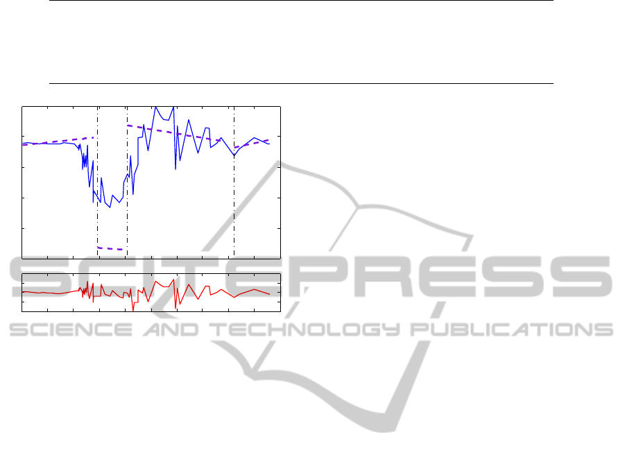
Table 1: Comparison of local performance of ANFIS and our method.

Model/Method ANFIS (training) Proposed (training) ANFIS (testing) Proposed (testing)

Local Model 1 63.6× 10

−3

7.5× 10

−3

55.5× 10

−3

12.0× 10

−3

Local Model 2 31.1× 10

−3

0.2× 10

−3

73.5× 10

−3

0.3× 10

−3

Local Model 3 349.5× 10

−3

7.4× 10

−3

276.8× 10

−3

25.0× 10

−3

Local Model 4 1.5× 10

−3

7.4× 10

−3

2.7× 10

−3

22.2× 10

−3

0 0.1 0.2 0.3 0.4 0.5 0.6 0.7 0.8 0.9 1

−0.5

−0.2

0.1

0.4

0.7

Acceleration (g)

Model

0 0.1 0.2 0.3 0.4 0.5 0.6 0.7 0.8 0.9 1

−0.4

−0.2

0.2

0.4

Overall error

Time (ms)

Figure 2: ANFIS model over the test dataset.

error of each dominant local model in its correspond-

ing time interval are listed in Table 1. This shows

that the local models obtained by ANFIS did not al-

ways give an accurate approximation within the local

regions. Note especially the eccentric behaviour of

submodel three (see Fig. 2 and Table 1). Fig. 1 and

the results in Table 1 conﬁrm that the method pro-

posed here led to an interpretable fuzzy neural model

with respect to all the local model behaviours. This

was not the case for the ANFIS method. Notice also

that the fourth local ANFIS model gave good results

due to the small (5) number of data points coupled

with the low noise in this time interval. Due to the

local characteristic of the weighted FRA, the hybrid

approach was also able to ﬁnd interpretable partitions

in a more complex problem than the one above. This

has not been included due to lack of space.

5 CONCLUSIONS AND FUTURE

WORK

In contrast to existing learning methods for fuzzy neu-

ral models which focus on the overall accuracy of

the model, and which may lead to uninterpretable ec-

centric behaviour in the local models, the aim here

has been to obtain a set of interpretable input space

partitions and the corresponding local models. Tak-

ing into account the two different parameter types

corresponded to the rule premise and rule conse-

quent, a new hybrid learning approach has been pro-

posed. This employed a modiﬁed differential evolu-

tion method to give the best fuzzy partitions, along

with a weighted fast recursive algorithm for identi-

ﬁcation of each local FLANN. An application study

and comparison with ANFIS illustrated the inter-

pretability of the resultant model structure and the

efﬁciency of the new learning technique. Further

improvements might accrue from investigating other

evolutionary strategies to optimize the rule premises.

ACKNOWLEDGEMENTS

The authors gratefully acknowledge the UK-China

Science Bridge grant EP/G042594/1, EP/F021070/1,

and the China Scholarship Council.

REFERENCES

Cheng, K. H. (2009). CMAC-based neuro-fuzzy ap-

proach for complex system modeling. Neurocomput-

ing, 72(7-9):1763–1774.

Li, K., Peng, J.X., and Irwin, G. W. (2005). A fast nonlinear

model identiﬁcation method. IEEE Transactions on

Automatic Control, 50(8):1211–1216.

Lin, C. J., Chen, C. H., and Lin, C. T. (2009). A hybrid

of cooperative particle swarm optimization and cul-

tural algorithm for neural fuzzy networks and its pre-

diction applications. IEEE Transactions on Systems,

Man, and Cybernetics, 39(1):55–68.

Qin, A. K. and Suganthan, P. N. (2005). Self-adaptive dif-

ferential evolution algorithm for numerical optimiza-

tion. In Proceedings of the IEEE congress on evolu-

tionary computation, volume 2, pages 1785–1791.

Silverman, B. W. (1985). Some aspects of the spline

smoothing approach to non-parametric regression

curve ﬁtting. Journal of the Royal Statistical Society

Series B, 47(1):1–52.

Storn, R. and Price, K. (1997). Differential evolution - A

simple and efﬁcient heuristic for global optimization

over continuous spaces. Journal of Global Optimiza-

tion, 11(4):341–359.

A HYBRID APPROACH TO LOCALLY OPTIMIZED INTERPRETABLE PARTITIONS OF FUZZY NEURAL

MODELS

465