DEVELOPMENTAL PLASTICITY IN CARTESIAN GENETIC

PROGRAMMING BASED NEURAL NETWORKS

Maryam Mahsal Khan, Gul Muhammad Khan

Electrical Engineering Department, University of Engineering and Technology, Peshawar, Pakistan

Julian F. Miller

Department of Electronics, University of York, York, U.K.

Keywords:

Generative and developmental approaches, NeuroEvolutionary algorithms, Pole balancing.

Abstract:

This work presents a method for exploiting developmental plasticity in Artiﬁcial Neural Networks using Carte-

sian Genetic Programming. This is inspired by developmental plasticity that exists in the biological brain

allowing it to adapt to a changing environment. The network architecture used is that of a static Cartesian

Genetic Programming ANN, which has recently been introduced. The network is plastic in terms of its dy-

namic architecture, connectivity, weights and functionality that can change in response to the environmental

signals. The dynamic capabilities of the algorithm are tested on a standard benchmark linear/non-linear control

problems (i.e. pole-balancing).

1 INTRODUCTION

Natural neural systems are not static in nature. They

interact and respond to environmental factors. Such

dynamic interactions lead to modiﬁcation or devel-

opment of the system with time. A static system

can be trained to give a speciﬁc response to a set

of environmental stimuli however it cannot learn or

adapt to a changing environment. To do this one

requires a network that develops at runtime. Evo-

lutionary computation based algorithms have proved

to be effective at ﬁnding a particular solution to a

computational problem, however, if the problem do-

main is slightly changed the evolved network is un-

able to solve the problem. Catastrophic forgetting

(CF) is the phenomenon in which a trained artiﬁcial

neural network loses its accuracy when the network

is trained again on a different computational prob-

lem (McCloskey and Cohen, 1989; Ratcliff, 1990;

Sharkey and Sharkey, 1995; Ans et al., 2002; French,

1994). Forgetting is inevitable if the learning resides

purely in the weights of ﬁxed connections.

Our aim is to ﬁnd a set of computational func-

tions that encode neural network architecture with an

ability to adapt to the changing environment as a re-

sult of development. Such plastic neural networks are

different from conventional ANN models as they are

constantly adjusting both topology and weights in re-

sponse to external environmentalsignals. This means,

that they can grow new networks of connections when

the problem domain requires it. The main motiva-

tion for such a new model is to arrive at a plastic

neural network model that can produce a single neu-

ral network that can solve multiple linear/non-linear

problems (i.e. not suffer from a phenomenon called

catastrophic interference). We think that this can be

acheived by arriving at a neural network model in

which new neural sub-structures automatically come

into existence when the network is exposed to new

learning scenarios.

In this paper we introduce a plastic neural network

based on the representation of Cartesian Genetic Pro-

gramming (Miller and Thomson, 2000) (PCGPANN).

The performance of this algorithms is tested on the

standard benchmark problem of pole-balancing for

both linear and non-linear conditions.

In Section 2 we will brieﬂy review the current de-

velopmental algorithms presented to date. Section 3

gives an overview of Cartesian Genetic Programming

(CGP). In section 4, we will provide an overview

of the standard CGPANN algorithm. Section 5 de-

scribes how self-modiﬁcation or developmental plas-

ticity could be embedded in the standard CGPANN

algorithm. Section 6 - 8 is the application of the algo-

449

Mahsal Khan M., Muhammad Khan G. and F. Miller J..

DEVELOPMENTAL PLASTICITY IN CARTESIAN GENETIC PROGRAMMING BASED NEURAL NETWORKS.

DOI: 10.5220/0003615204490458

In Proceedings of the 8th International Conference on Informatics in Control, Automation and Robotics (ANNIIP-2011), pages 449-458

ISBN: 978-989-8425-74-4

 2011 SCITEPRESS (Science and Technology Publications, Lda.)

rithm on a standard benchmark problem - single and

double pole-balancing along with results and discus-

sion. Section 9 concludes with the ﬁndings and future

work.

2 RELATED WORK

GP has been used in a number of ways to produce

ANNs. The simplest of all is using direct encoding

schemes in which GP is used to encode the weights

of ANN or architecture or both. In direct encoding

schemes each and every unit in phenotype is speciﬁed

in the genotype. Specifying each connection of ANN

in genotype is commonly referred to as ‘structural en-

coding’ (Hussain and Browse, 2000).

Another important form of encoding that is used

to develop ANNs is Grammar encoding. There are

two types of grammar encoding schemes: develop-

mental grammatical encoding and derivation gram-

matical encoding. Kitano used developmental gram-

matical encoding scheme for development of ANN

(Kitano, 1990). In this, genes describe the grammat-

ical rule that is used for development of the ANN. In

derivation grammatical encoding, the gene contains

a derivation sequence that specify the whole network

(Gruau, 1994; Jacob and Rehder, 1993).

Cellular Encoding (CE) devised by Gruau et.al

(Gruau et al., 1996) is a developmental neuroevolu-

tionary algorithm. Weights, connection, graph re-

writing rules are evolved based on the evolutionary

algorithm. CE transforms graph in a manner that con-

trols cell division which grows into an ANN. CE was

applied on a control problem of balancing single and

double poles. This technique was found to scale bet-

ter and was effective at optimizing both architecture

and weights together.

A model proposed by Nolﬁ et.al maps a genotype

into a phenotype during the existence of the individ-

ual. The life expectancy of the individual is affected

by the external environment and the genotype itself

(Nolﬁ et al., 1994). The two dimensional neural net-

work adapts during their lifetime as environmental

conditions affect the growth of the axons. The neu-

rons had only upward growing axons with no den-

drites.

The development of a neural architecture from

a single cell was proposed by Cangelosi. In this

model the cell undergoes cell division and migra-

tion to produce a two dimensional neural architecture

(Cangelosi et al., 1994). The rules for both the pro-

cess of cell division and migration is speciﬁed in the

genotype; see (Dalaert and Beer, 1994; Gruau, 1994)

for related approaches.

Another developmentalmodel that evolves param-

eters based on genetic algorithm was proposed by

Rust and Adams. The evolved parameters represented

neurons that were biologically realistic. They also in-

vestigated the inﬂuence of dependent mechanisms on

growing morphologies of neuron (Rust et al., 2000).

Karl Sims used a graph based GP approach to

evolve virtual robotic creatures. The neural architec-

ture for controlling the body parts of the robots were

genetically determined (Sims, 1994).

Rogen et.al proposed a developmental spiking

ANN cellular model. Each cell is composed of an ex-

citory or inhibitory weight input neurons. The neuron

triggers once a certain threshold is reached and goes

into a short refractory period. Because of the leak-

age mechanism in spiking ANN, the threshold of the

membrane reduces with time (Roggen et al., 2007).

Rivero, evolved a specially designed tree-

representation which could produced an ANN graph

(Rivero et al., 2007). He tested his network on a num-

ber of data mining applications.

Harding et al. adapted the graph-based genetic

programming approach, known as Cartesian Genetic

Programming (CGP) by introducing a number of in-

novations. Foremost of which was the introduction

of self-modifying functions. The method is called

self-modifying CGP (SMCGP) (Harding et al., 2010).

Self-modifying functions allow an arbitrary number

of phenotypes to be encoded in a single genotype.

SMCGP was evaluated on a range of problems e.g.

digital circuits, pattern and sequence generation and,

notably, was found to produce general solutions to

some classes of problem (Harding et al., 2010).

Khan et al. presented a neuro-inspired devel-

opmental model using indirect encoding scheme to

develop learning neural architectures (Khan et al.,

2007). They used cartesian genetic programming to

encode a seven chromosome neuron genotype. The

programs encoded controlled the processing of sig-

nals and development of neural structures with mor-

phology similar in certain ways to biological neurons.

The approach has been tested on a range of AI prob-

lems including: Wumpus world, Solving Mazes and

the Game of Checkers (Khan et al., 2007).

The N-gram GP system is extended to incorporate

developmental plasticity known as ‘Incremental Fit-

ness based Development (IFD)’ proposed by McPhee

et.al (Nicholas F.McPhee and Poli, 2009). Both N-

gram and IFD have been applied on various regres-

sion problems where IFD has been found producing

better results.

HyperNEAT is one of the indirect encoding strate-

gies of developmental ANNs (Stanley et al., 2009).

HyperNEAT uses generative encoding and the basic

ICINCO 2011 - 8th International Conference on Informatics in Control, Automation and Robotics

450

evolutionary principles based on the NEAT (Neuro

Evolution of Augmented Topology) algorithm (Stan-

ley and Miikkulainen, 2002). In HyperNEAT the

weights(inputs) are presented to an evolved program

called a Compositional Pattern Producing Networks

(CPPNs). The CPPN takes coordinates of neurons in

a grid and outputs the corresponding weight for that

connection. The algorithm has been applied to Robot

locomotion. Regular quadruped gaits in the legged lo-

comotion problem have been successfully generated

using this algorithm (Clune et al., 2008).

Synaptic plasticity in Artiﬁcial neural network can

be introduced by using local learning rules that mod-

ify the weights of the network at runtime (Baxter,

1992). Floreano and Urzelai have demonstrated that

evolving network with synaptic plasticity can solve

complex problemsbetter than recurrent networks with

ﬁxed-weights (Floreano and Urzelai, 2000). A num-

ber of researchers have investigated and compared the

performance of plastic and recurrent networks obtain-

ing mixed results with either of them performing bet-

ter in various problem domains (for a review see (Risi

et al., 2010)). One of the interesting features of the ap-

proach we propose is that, unlike previous approaches

investigated, it has both synaptic and developmental

plasticity.

3 CARTESIAN GENETIC

PROGRAMMING

Cartesian Genetic Programming (CGP) is an evo-

lutionary technique for evolving graphs (Miller and

Thomson, 2000). The graphs are arranged in the

form of rectangular grids like multi-layer percep-

trons. The graph topology is deﬁned using three pa-

rameters: number of columns, number of rows and

levels-back. The number of nodes in the graph en-

coded in the genotype is the product of the number

of columns and the number of rows. Usually feedfor-

ward graphs are evolved in which inputs to a node are

the primary inputs or outputs from the previous nodes.

The levels-back parameter constrains connections be-

tween nodes. For instance, if levels-back is one, all

nodes can only be connected to nodes immediately

preceeding them, while if levels-back is equal to the

number of columns of nodes (primary inputs are al-

lowed to disobey this constraint) the encoded graphs

could be an arbitrary feed-forward graph. Genotypes

consist of a ﬁxed length string of integers (referred to

as genes). These genes represents nodes with inputs

and functions. Functions can be any linear/non linear

functions. The output of the genotype can be from

any node or the primary inputs. CGP generally uses a

1+4 evolutionary strategy to evolve the genotype. In

this the parent genotype is unchanged and 4 offspring

are produced by mutating the parent genotype. It is

important to note that when genotypes are decoded

nodes may be ignored as they are not connected in

the path from inputs to outputs. The genes associated

with such nodes are non-coding. This means that the

active ﬁnal graph encoded could consist of a pheno-

type containing any subset of number of nodes de-

ﬁned in the genotype. Mutating a genotype can thus

change the phenotype either not at all or drastically.

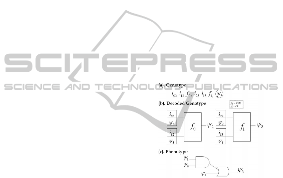
We give a simple example of CGP in Figure.1

where 1(a) shows a 1x2 (rows x columns) geno-

type for a problem with 2 binary inputs ‘ψ

0,1

’ and

1 binary output. The inputs to each node is repre-

sented as i

where ‘m’ represents the input from

and ‘n’ is the input to the node. The functions ‘f

’

used are logical ‘OR’ and logical ‘AND’. Figure.1(b)

shows the graphical representation of the genotype

in Figure.1(a). The resultant phenotype shown in

Figure 1: (a) CGP based Genotype for a problem with 2

binary inputs ψ

and ψ

. Single program output is taken

from the last gene (circled). (b) Decoding of the genotype.

Figure.1(c) can be represented as a logical equation

in Eq.(1) where ‘+’ represent OR and ‘.’ represents

AND operation.

= ψ

.ψ

+ ψ

(1)

4 CGP EVOLVED ANN

The representation of CGP has been exploited in gen-

erating static neural architectures. Both feedforward

and recurrent (FCGPANN , RCGPANN) based net-

works have been designed and tested on various ap-

plications (Khan et al., 2010b; Khan et al., 2010a).

DEVELOPMENTAL PLASTICITY IN CARTESIAN GENETIC PROGRAMMING BASED NEURAL NETWORKS

451

In CGPANN, along with standard CGP genes (in-

puts, functions) weight and switch genes are also in-

troduced. The weight values are randomly assigned to

each input with values from (−1,+1). Switch genes

are either ‘1’ or ‘0’ where ‘1’ is a connected and ‘0’ a

disconnected input. The genotype is then evolved to

obtain best topology, optimal weights and combina-

tion of functions.

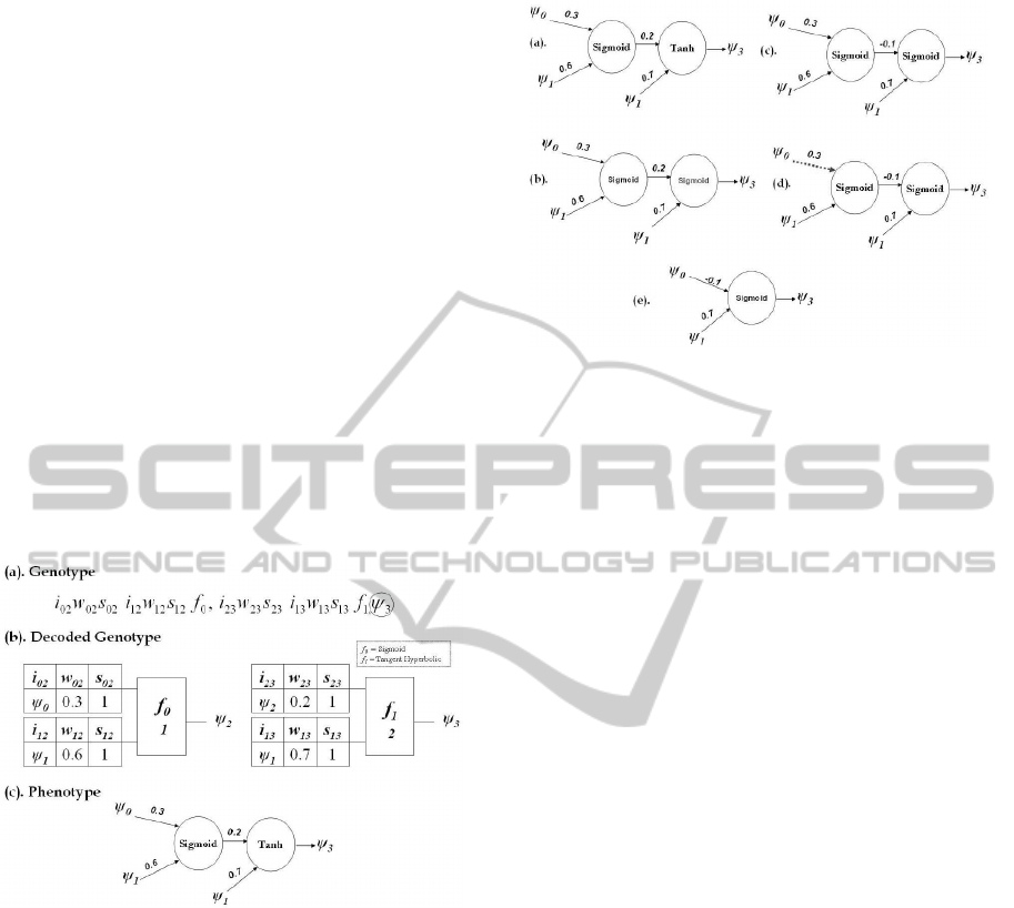
Figure.2 is an example of a CGPANN genotype

with two primary inputs ψ

0,1

and one output. The

activation function f

used are sigmoid and tangent

hyperbolic. The inputs to each node is represented as

. Similarly weights w

are assigned to each in-

put. Whether an input is connected or not is encoded

as a switching gene s

. Figure.2(a) is the genotype

of a 1x2 architecture with the output taken from node

. Figure.2(b) is the graphical view of the genotype

with values assigned e.g. the weight assigned to the

input i

supplied to node 2 is w

= 0.6. The pheno-

type of the genotype is shown in Figure.2(c) which is

mathematically expressed in Eq.(2).

Figure 2: (a) Genotype of a 1x2 architecutre with two in-

puts. (b) Decoded Genotype. (c) Phenotype represented as

ANN of the genotype.

= Tanh(0.7ψ

+ 0.2sig(0.3ψ

+ 0.6ψ

)) (2)

5 PLASTIC CGP NEURAL

NETWORK

A plastic CGPANN (PCGPANN) is a developmental

form of Cartesian Genetic Programming ANN algo-

rithm. The basic structure and representation of the

PCGPANN is similar to the CGPANN structure as

shown in Figure. 2. In the PCGPANN method, an

additional output gene is added to the genotype. It is

used for making developmental decisions. According

to whether the output value is less than zero or above,

Figure 3: PCGPANN - Plastic Development of Neural Net-

work Parameters (a) Initial Phenotype. (b) Mutation of

Function. (c) Mutation of Weight. (d) Mutation of Switch.

(e) Mutation of Input.

a ‘mutation’ of the genotype is introduced to create

a new phenotype. In this way, a single genotype can

evoke an unlimited series of phenotypes depending

on the real-time output of the program encoded in the

genotype. The modiﬁcation of the genotype results

in different phenotypic structures. The mutation pro-

duced is randomly chosen from the types listed below.

It should be noted that some gene changes may result

in no phenotypic change as in CGP many genes are

redundant. The phenotypic mutation of neural net-

work can be any of the following: inputs, weights,

switches,outputs and activation functions. Genes are

mutated and assigned a valid value based on sets of

constraints.

• If a gene represents a function then it is replaced

by any random function selected from 1 to total

number of functions (n

) available to the system.

• If the gene represents a weight is replaced by a

weight value between (-1, +1).

• If the gene is a switching gene then it is comple-

mented.

• Node input genes are mutated by assigning an in-

put value such that the levels-back parameter is

still obeyed.

• An output can be assigned any random value from

1 to total number of nodes plus inputs presented to

the system.

Figure.3 shows a step by step process of mutation

on a phenotype. Figure.3(a) is the initial phenotype

of the genotype given in Figure.2(c). As in the de-

scribed example the activation functions used were

two - sigmoid and tangent hyperbolic. Thus the geno-

type has only two functions to randomly choose from.

ICINCO 2011 - 8th International Conference on Informatics in Control, Automation and Robotics

452

In Figure.3(b) the function is mutated from tangent

hyperbolic to sigmoid . The mathematical expression

of the updated genotype is thus changed as shown in

Eq.(3).

= sig(0.7ψ

+ 0.2sig(0.3ψ

+ 0.6ψ

)) (3)

Figure.3(c) represents a mutated phenotype where the

value of weight is changed from 0.2 to -0.1 expressed

in Eq.(4).

= sig(0.7ψ

− 0.1sig(0.3ψ

+ 0.6ψ

)) (4)

Similarly Figure.3(d) displays the mutated phenotype

where the switching gene is toggled and switched off

(shown as dotted line). Thus the input is no longer

connected to the node. Mathematically expressed by

Eq.(5).

= sig(0.7ψ

− 0.1sig(0.6ψ

)) (5)

Mutation of inputs is one of the major tunning pa-

rameter during the developmental process of ANN.

From the phenotype displayed in Figure.3(d), the in-

put to the second node is ψ

and an output from the

ﬁrst node. After mutating the input, the input to the

second node is modiﬁed to two primary inputs of the

system ψ

0,1

. The resultant phenotype is displayed

in Figure.3(e) with its function in Eq.(6). Thus dur-

ing runtime different functional equations can be pro-

duced generating desired response.

= sig(−0.1ψ

+ 0.7ψ

) (6)

Similarly output of any genotype can also be mutated

and changed to another node. In this way inactive

genes present in the genotype can be activated or vice

versa. This in turn effects the phenotypic structure of

the genotype.

It is worth mentioning here that mutation of geno-

type at runtime affects only a single gene where as

mutation from generation to generation is dependent

on the mutation rate ﬁxed at the start of the program,

thus changing the starting genotype for each develop-

ment.

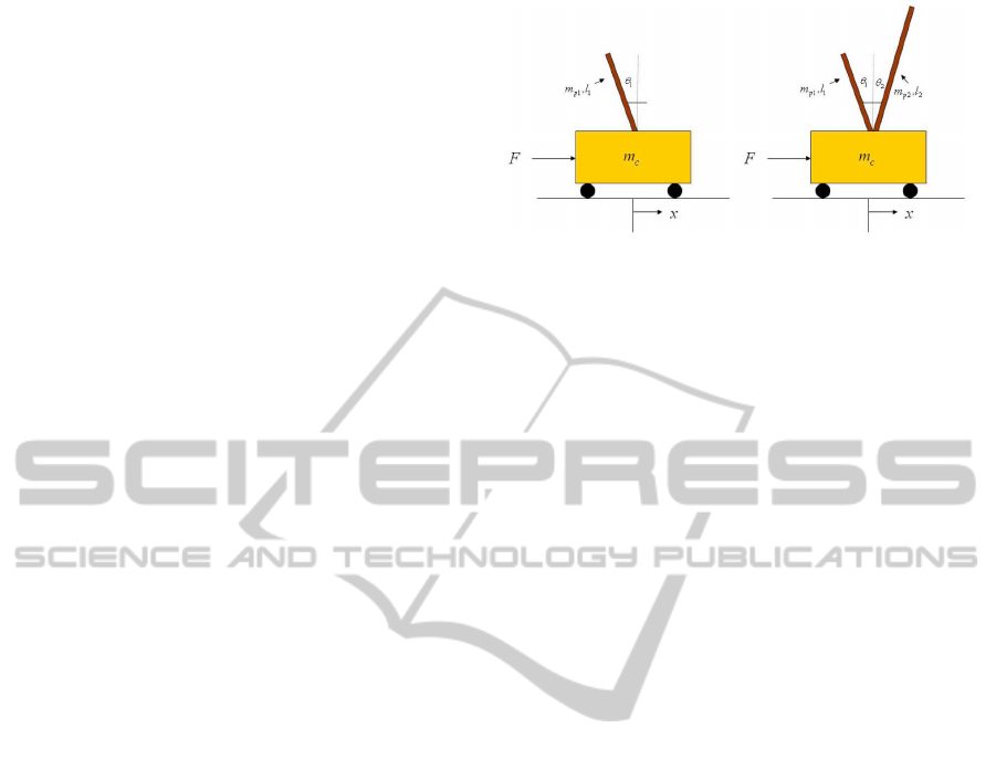
6 CASE STUDY: BALANCING

POLE(S)

Pole balancing also known as inverted pendulum is

a standard benchmark problem in the ﬁeld of control

theory. The performance of various neuroevolution-

ary algorithms is tested on this problem. Single pole

balancing task consists of a pole attached by a hinged

to a wheel cart while double pole balancing consti-

tutes two poles. In both the cases the track of the cart

Figure 4: (a) Single Pole Balancing. (b) Double Pole Bal-

ancing.

is limited to −2.4 < x < +2.4 as shown in Figure.4.

The objective is to apply force ‘F’ to the cart such

that the cart doesn’t leave the track and the angle of

the pole doesn’t exceed (-12

◦

< θ

< +12

◦

) for single

pole and (-36

◦

< θ

1,2

< +36

◦

) for the double pole bal-

ancing task. The controller has to balance the pole(s)

for approximately 30 minutes which corresponds to

100,000 time steps. Thus the neural network must ap-

ply force to the cart to keep the pole(s) balanced for as

long as possible. The input to the system are the angle

of pole(s) (θ

1,2

), angular velocity of pole (

1,2

), posi-

tion of cart (x) and velocity of cart (˙x). Equations that

are used to compute the effective mass of poles, accel-

eration of poles, acceleration of cart, effective force

on each pole, the next state of angle of poles, veloc-

ity of poles, position of cart and velocity of cart along

with the parameters deﬁned for both control problems

can be found in (Khan et al., 2010a).

7 EXPERIMENTAL SETUP

PCGPANN genotypes are generated for various net-

work sizes for both single and double pole balanc-

ing task. A mutation rate of µ

= 10% is used for

all the networks. The activation functions f

used

are sigmoid and tangent hyperbolic. Each genotype

is initialized with random weights ‘w’ from -1 to +1,

switching ‘s’ values of 0 or 1 and random inputs ‘ψ

’.

The number of outputs ‘O

’ from the system are 2 i.e.

and O

. Both the outputs are normalized between

-1 to +1. Output O

represents the ‘Force (F)’ that

controls the force applied to the cart and the output

is associated with the developmental plasticity of

the network. Using one of the outputs of the genotype

for making developmental decision acts as a feedback

to the system for generating plastic changes.

We have simulated the network for two develop-

mental strategies Dev

and Dev

as shown in Eq.(7)-

(8). Both the strategies are tested on the pole bal-

ancing task for single and double pole(s) with zero

DEVELOPMENTAL PLASTICITY IN CARTESIAN GENETIC PROGRAMMING BASED NEURAL NETWORKS

453

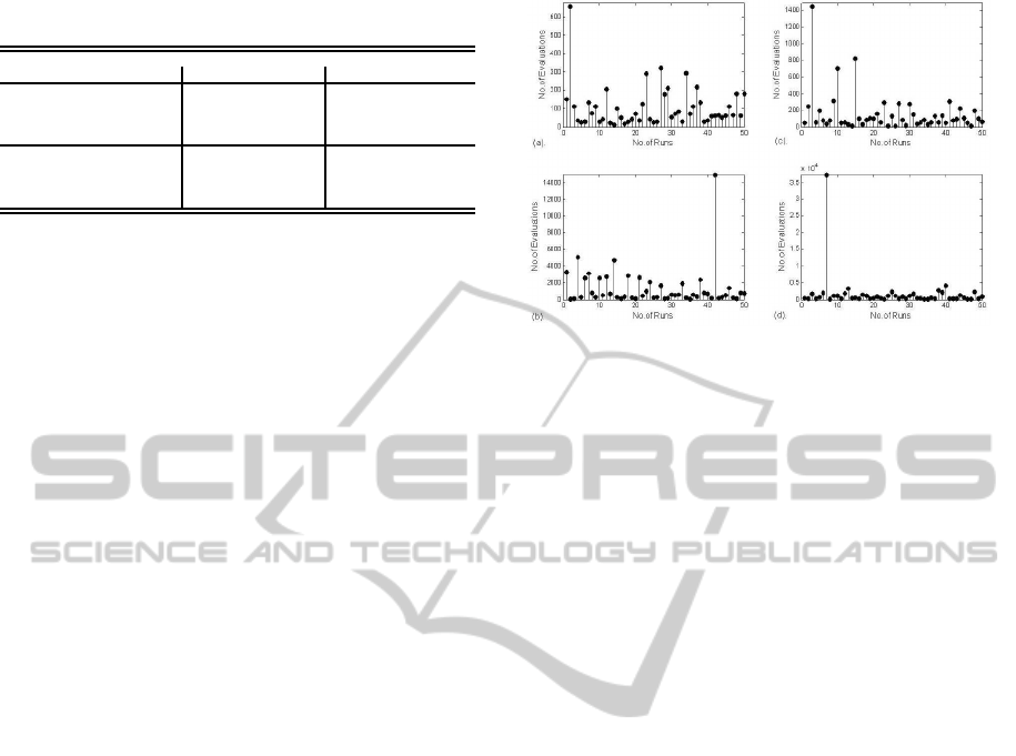
Table 1: Performance of PCGPANN on Single and Double

Poles.

Network Representation SinglePole Evaluations DoublePole Evaluations

Initial State Network Arch. Dev

Dev

Zero 4x4 221 659 1716 6310

5x5 186 570 1169 5494

10x10 104 519 1337 8315

15x15 168 643 1934 7334

Random 4x4 390 608 1738 3310

5x5 303 387 1981 4033

10x10 157 243 1612 3308

15x15 160 260 1916 4362

and random initial states. The intention is to identify

faster and robust strategies for the problem investi-

gated.

Dev

(

No −Change -1 ≤ O

≤ 0

Mutation− of − Parameters 0< O

≤ 1

(7)

Dev

(

Mutation− of − Parameters -1 ≤ O

≤ 0

No −Change 0< O

≤ 1

(8)

7.1 Single Pole: Zero and Random

Initial States

In single pole balancing the input to the networks are

position of cart x, velocity of cart ˙x, angle of pole θ

and velocity of pole

. The number of inputs to each

node is taken as 4, which is equivalent to the number

of inputs to the system.

7.2 Double Pole: Zero and Random

Initial States

Double pole balancing involves balancing an addi-

tional pole. The number of input to the networks are

position of cart x, velocity of cart ˙x, angle of poles θ

1,2

and angular velocity of poles

1,2

. The number of in-

put to each node is taken as 6, which is equivalent to

the number of inputs to the system.

In both the cases (single and double poles), the

networks are generated with initial input values of

zero or with random values of -0.25rad <θ

<0.25rad

and -2.4 <x <+2.4 for single pole and -0.6rad <θ

1,2

<0.6rad and -2.4 <x <+2.4 for double poles. The

performance of the PCGPANN algorithm is based on

the average number of balancing attempts (evalua-

tions) for ﬁfty independent evolutionary runs.

8 RESULTS AND DISCUSSIONS

Table 1 represents average number of balancing at-

tempts for inputs starting from initial states of zero

and random states of network with varying network

Figure 5: Variation in the number of evaluations of the

best evolved network’s genotypes for single(a,c) and dou-

ble poles(b,d) with zero and random initial states.

sizes for single and double pole(s) balancing tasks

under both the developmental strategies. The results

are the average of 50 independent evolutionary runs.

Figure.5 shows the variation in the number of evalua-

tions of the best evolved network’s genotypes for sin-

gle/double pole(s) with zero and random initial states.

From the ﬁgure it is evident that out of ﬁfty genotypes

only one of them took longer than expected number

of evaluations thus increasing the overall average. It

is observed in all the four cases of Figure.5 that learn-

ing speed is much faster in 98% of the evolutionary

runs. It is observed in Table 1 that the developmen-

tal strategy Dev

has performed better than the Dev

strategy for both the single and double pole balancing

tasks. From Table 1, the minimum average evalua-

tions of 50 independent runs for the single pole and

double pole was 104 and 1169 respectively. Random

initial states took longer time to develop into a stable

structure as compared to zero initial states for obvi-

ous reasons. For both single and double pole balanc-

ing task, fast learning in terms of minimum average

evaluations has been found in the 10x10 network ar-

chitecture.

Figure.6 represents the pole angles and position of

cart simulated for 30 minutes respectively (100,000

steps are down-sampled to produce 100 steps for

demonstration purpose only) for the single pole and

double pole balancing task. In Figure.6(a) the cart

is moving back and forth to make the pole bal-

anced while minute changes in the angle of pole

is observed. Similarly in case of Figure.6(b) ran-

dom behaviour of movement of both the poles and

the cart is observed for the double pole balancing

task. Pole balancing task is used as a benchmark

by researchers to investigate the performance of al-

gorithms including: Conventional Neuro Evolution

(CNE) (Wieland, 1991), Symbiotic, Adaptive Neural

ICINCO 2011 - 8th International Conference on Informatics in Control, Automation and Robotics

454

Figure 6: Pole Angle(s) and Position of Cart simulated for 100,000 steps for (a) Single Pole Task (b) Double Pole Task.

Table 2: Comparison of PCGPANN with other neuroevolu-

tionary algorithms Applied on Single and Double Pole Bal-

ancing Task: average number of network evaluations.

Method SinglePole DoublePole

CNE 352 22100

SANE 302 12600

ESP 289 3800

NEAT 743 3600

CoSyNE 98 954

FCGPANN 21 77

PCGPANN 104 1169

Evolution (SANE)(Moriarty, 1997), Enforced Sub-

Population (ESP) (Gomez and Miikkulainen, 1999),

Neuro Evolution of Augmenting Topologies (NEAT)

(Stanley and Miikkulainen, 2002) and Cooperative

synapse neuroevolution (CoSyNE) (Gomez et al.,

2008). All these neuroevolutionary algorithms pro-

duces static ANNs detail of which can be found in

(Khan et al., 2010a). Table 2 represents the compar-

ison of performance of the Plastic CGPANN with all

these neuroevolutionary algorithms for both the sin-

gle and double pole balancing tasks. Developmen-

tal CGPANN has outperformed most of these neu-

roevolutionary algorithms by quite a large margin. As

pointed out by Risi et al. learning a speciﬁc task is

easy but learning the strategy to learn and adapting

its architecture to the changing task takes time (Risi

et al., 2010). This is the reason that PCGPANN took

more evaluations to arrive at a solution as compared to

its static counterpart - FeedForward CGPANN (FCG-

PANN)(Khan et al., 2010a).

8.1 Developmental Plasticity

It is observed in the CGP literature that only upto 5%

nodes are usually active at runtime, thus having 95%

of garbage space (inactive nodes) that may be acti-

vated during evolution (Miller and Smith, 2006). As

the overall architecture of the system in PCGPANN

is ﬁxed (5x5, 10x10, etc networks), only the inter-

connectivity of the neurons changes at runtime thus

changing the active morphology of the ultimate phe-

notype. This phenomenon is similar to what is ob-

served in biological brain with different parts of ner-

vous system responding to different sets of input at

runtime (Kandel et al., 2002). In Plastic CGPANN

algorithm neurons are presented in terms of network

sizes where a 5x5 network corresponds to 25 neu-

rons. The target is then to use these neurons like re-

sources in a system in an effective and efﬁcient man-

ner. The structure produced connects and disconnects

during the developmental process generating differ-

ent sets of equations at run time. This corresponds to

the creation of different phenotypes during a genera-

tion, similar to the work done by Nolﬁ (Nolﬁ et al.,

1994). Such plasticity embeds efﬁcient utilization of

resources and reduces hardware cost. Till date no

developmental algorithm other than PCGPANN have

been proposed that has excessive neuron structures

that activate and deactivate with time rather ﬁx ar-

chitectures are mostly proposed. Figure.7 shows the

logarithmic graphs for developmental outputs of six

different evolved genotypes for both the developmen-

tal strategies while balancing double poles for 30mins

(100,000 time steps). It is evident from these graphs

that after some early development the ultimate output

of the network causes the network to stay same (no

change decision). It can be seen in Figure.7(a,c,e)that

genotypes produces developmental output with oscil-

lating behaviour at the beginning resulting in change

of phenotypic structure and weights more often. Sim-

ilar behaviour is also observed in biological brain

where most of the learning and development happens

in the immature brain as compared to the adult brain.

Hence changing or mutating parameters at the early

stage has greater probability of convergence to the so-

lution.

Figure.8 shows the statistics of various param-

DEVELOPMENTAL PLASTICITY IN CARTESIAN GENETIC PROGRAMMING BASED NEURAL NETWORKS

455

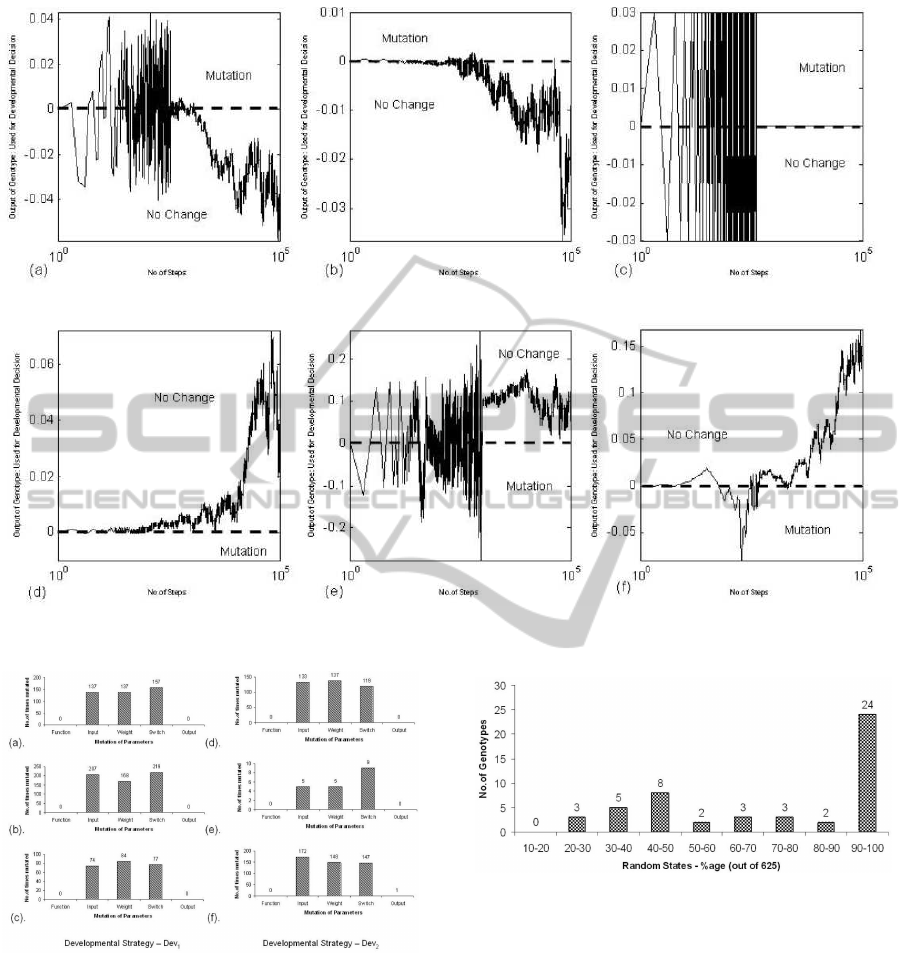
Figure 7: Developmental Behaviour of the network - (a,b,c) Dev

Strategy and (d,e,f) Dev

strategy.

Figure 8: Statistics of the changes in network parameters

for the six cases in Figure 7.

eters that are mutated for the six cases in Figure.7

during 100,000 time steps while the pole(s) are be-

ing balanced. A similar trend is observed in all the

cases with switches, inputs and weights updated with

almost same ratio. On average the network is changed

by 0.3 to 0.4% during runtime with most (95%) devel-

opment taking place at the early stage as evident from

Figure.7.

As learning to learn is a complex dynamic nonlin-

Figure 9: SinglePole Task-Number of Genotypes that are

successful in balancing the pole in 625 random initial states.

ear process even a biological brain does not process

inputs linearly. Remaining dormant for a number of

steps reduces the chance of quick learning while it is

observed that changing and adapting (to remain dor-

mant) to the change is an effective strategy of learn-

ing.

8.2 Robustness of PCGPANN

The robustness of the genotypes is inferred by sub-

jecting the genotype to 625 random initial states and

checking it for 1000 steps only. If the genotype is

able to balance then it is termed as robust. Figure.

ICINCO 2011 - 8th International Conference on Informatics in Control, Automation and Robotics

456

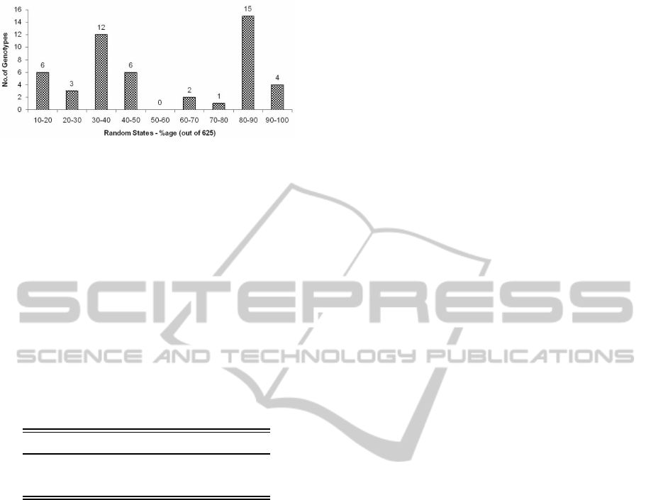
Figure 10: DoublePole Task-Number of Genotypes that are

successful in balancing the pole in 625 random initial states.

9 and 10 represents the performance of 50 genotypes

(solutions of the single and double pole task) on 625

random initial states. For the single pole, 48% of

the genotype were able to balance at 90-100% (which

corresponds to 563-625) of the random states which

can be inferred from the graph presented in Figure.9,

thus attaining an average of 456. While for the dou-

ble pole 44% genotypes were able to balance at 60-

100% of the random states achieving an average of

349. Thus the genotypes undergoing developmental

plasticity during the 1000 steps exhibit robustness.

Table 3: Average number of random cart-pole initializations

(out of 625) that can be solved.

Type SinglePole DoublePole

FCGPANN 590 277.38

PCGPANN 456 349

Table.3 shows the generalization of the PCG-

PANN genotypes in comparison to feedforward CG-

PANN for both the single and double pole balancing

scenarios. The PCGPANN strategy proves more ro-

bust in the double pole balancing task (which is a non-

linear problem) where on average a genotype at 349

out of 625 different initial states is developed into suc-

cessful and feasible solutions.

9 CONCLUSIONS

In this paper, plastic feedforward neural network

based on the representation of Cartesian Genetic Pro-

gramming (PCGPANN) is proposed and applied on

a standard benchmark control problems. Plastic-

ity involves mutating the neural network parameters

namely weight, switches, inputs, functions and out-

put at run-time. Plastic/Developmental decisions are

made by using a developmental output from the net-

work which induces plastic changes at runtime. The

neurocontrollers produced by PCGPANN algorithm

were found to be more robust than its FCGPANN

counterpart. The network phenotype changes during

run time, thus modifying its architecture in response

to changing input patterns. The algorithm was also

found to outperform most of the static neuroevolu-

tionary algorithms in terms of speed of learning. It

should be noted that the phenotypic mutations happen

each time the new output is obtained from the evolved

program in the genotype. However, in principle, this

could be done at a slower rate (for instance, after a

certain number of evolved program executions, rather

than at every timestep). This remains to be investi-

gated.

In future plasticity will be investigated for recur-

rent networks and tested for the non-markovian con-

trol problems. The goal is to investigate whether in-

duction of both signal based feedback (recurrent) and

structural feedback (plasticity) can enhance the per-

formance. Also we intend to examine whether the

PCGPANN is able to solve problems faster and more

accurately by obtaining repeated experienceof its task

environment (post evolution). Eventually the aim is

to investigate whether PCGPANNs can be trained to

solve a sequence of problems without forgetting how

to solve earlier problems.

REFERENCES

Ans, B., Rousset, S., French, R. M., and Musca, S.

(2002). Preventing catastrophic interference in

multiple-sequence learning using coupled reverberat-

ing elman networks. In Proc. 24th, Annual conf. of

cognitive science society, pages 71–76.

Baxter, J. (1992). The evolution of learning algorithms for

artiﬁcial neural networks. D.Green & T.Bossomaier,

Complex Systems, pages 313 – 326.

Cangelosi, A., Nolﬁ, S., and Parisi, D. (1994). Cell division

and migration in a ’genotype’ for neural networks.

Network-Computation in Neural Systems, 5:497–515.

Clune, J., Beckmann, B. E., Ofria, C., and Pennock,

R. T. (2008). Evolving coordinated quadruped gaits

with the hyperneat generative encoding. Proc. IEEE

CEC’2008, pages 2764–2771.

Dalaert, F. and Beer, R. (1994). Towards an evolvable

model of development for autonomous agent synthe-

sis. In Brooks, R. and Maes, P. eds. Proc. 4rth Conf.

on Artiﬁcial Life. MIT Press.

Floreano, D. and Urzelai, J. (2000). Evolutionary robots

with online self-organization and behavioral ﬁtness.

Neural Networks, 13:431 – 443.

French, R. M. (1994). Catastrophic forgetting in connec-

tionist networks: Causes, consequences and solutions.

In Trends in Cognitive Sciences, pages 128–135.

DEVELOPMENTAL PLASTICITY IN CARTESIAN GENETIC PROGRAMMING BASED NEURAL NETWORKS

457

Gomez, F., Schmidhuber, J., and Miikkulainen, R. (2008).

Accelerated neural evolution through cooperatively

coevolved synapses. J. Mach. Learn. Res., 9:937–965.

Gomez, F. J. and Miikkulainen, R. (1999). Solving non-

markovian control tasks with neuroevolution. In Proc.

Int. joint Conf. on Artiﬁcial intelligence, pages 1356–

1361. Morgan Kaufmann Publishers Inc.

Gruau, F. (1994). Automatic deﬁnition of modular neural

networks. Adaptive Behaviour, 3:151–183.

Gruau, F., Whitley, D., and Pyeatt, L. (1996). A com-

parison between cellular encoding and direct encod-

ing for genetic neural network. In Genetic Program-

ming 1996:Proceeding of the First Annual conference,

pages 81–89 MIT Press.

Harding, S., Miller, J. F., and Benzhaf, W. (2010).

Developments in cartesian genetic program-

ming:selfmodifying cgp. GPEM, 11(2):397–439.

Hussain, T. and Browse, R. (2000). Evolving neural net-

works using attribute grammars. IEEE Symp. Combi-

nations of Evolutionary Computation and Neural Net-

works, 2000, pages 37 – 42.

Jacob, C. and Rehder, J. (1993). Evolution of neural

net architectures by a hierarchical grammar-based ge-

netic system. In Proc. ICANNGA93, pages 72–79.

Springer-Verlag.

Kandel, E. R., Schwartz, J. H., and Jessell (2002). Princi-

ples of Neural Science, 4rth Edition. McGraw-Hill.

Khan, G., Miller, J., and Halliday, D. (2007). Coevolution

of intelligent agents using cartesian genetic program-

ming. In Proc. GECCO’2007, pages 269 – 276.

Khan, M., Khan, G., and F. Miller, J. (2010a). Evolution

of optimal anns for non-linear control problems us-

ing cartesian genetic programming. In Proc. IEEE.

ICAI’2010.

Khan, M., Khan, G., and Miller, J. (2010b). Efﬁ-

cient representation of recurrent neural networks for

markovian/non-markovian non-linear control prob-

lems. In Proc. ISDA’2010, pages 615–620.

Kitano, H. (1990). Designing neural networks using ge-

netic algorithm with graph generation system. Com-

plex Systems, 4:461–476.

McCloskey, M. and Cohen, N. (1989). Catastrophic in-

terference in connectionist networks: The sequential

learning problem. The Psychology of Learning and

Motivation, 24:109–165.

Miller, J. and Smith, S. (2006). Redundancy and com-

putation efﬁciency in cartesian genetic programming.

IEEE Trans. Evol. Comp., 10:167–174.

Miller, J. F. and Thomson, P. (2000). Cartesian genetic

programming. In Proc. EuroGP’2000, volume 1802,

pages 121–132.

Moriarty, D. (1997). Symbiotic Evolution of Neural Net-

works in Sequential Decision Tasks. PhD thesis, Uni-

versity of Texas at Austin.

Nicholas F.McPhee, Ellery Crane, S. E. and Poli, R. (2009).

Developmental plasticity in linear genetic program-

ming. Proc. GECCO’2009, pages 1019–1026.

Nolﬁ, S., Miglino, O., and Parisi, D. (1994). Phenotypic

plasticity in evolving neural networks. In Proc. Int.

Conf. from perception to action. IEEE Press.

Ratcliff, R. (1990). Connectionist models of recognition

and memory:constraints imposed by learning and for-

getting functions. Psychological Review, 97:205–308.

Risi, S., Hughes, C. E., and Stanley, K. O. (2010). Evolving

plastic neural networks with novelty search. Adaptive

Behavior.

Rivero, D., Rabual, J., Dorado, J., and Pazos, A. (2007).

Automatic design of anns by means of gp for

data mining tasks: Iris ﬂower classiﬁcation prob-

lem. Adaptive and Natural Computing Algorithms,

4431:276–285.

Roggen, D., Federici, D., and Floreano, D. (2007). Evo-

lutionary morphogenesis for multi-cellular systems.

GPEM, 8:61–96.

Rust, A., Adams, R., and H., B. (2000). Evolutionary neural

topiary: Growing and sculpting artiﬁcial neurons to

order. In Proc. ALife VII, pages 146–150. MIT Press.

Sharkey, N. and Sharkey, A. (1995). An analysis of catas-

trophic interference. Connection Science, 7(3-4):301–

330(30).

Sims, K. (1994). Evolving 3d morphology and behavior

by competition. In Artiﬁcial life 4 proceedings, pages

28–39. MIT Press.

Stanley, K. O., D’Ambrosio, D. B., and Gauci, J. (2009).

A hypercube-based encoding for evolving large-scale

neural networks. Artif. Life, 15:185–212.

Stanley, K. O. and Miikkulainen, R. (2002). Evolving neu-

ral network through augmenting topologies. Evolu-

tionary Computation, 10(2):99–127.

Wieland, A. P. (1991). Evolving neural network controllers

for unstable systems. In Proc. Int. Joint Conf. Neural

Networks, pages 667–673.

ICINCO 2011 - 8th International Conference on Informatics in Control, Automation and Robotics

458