
WORKFLOW COMPOSITION AND DESCRIPTION TOOL
Binh Minh Nguyen, Viet Tran and Ladislav Hluchy
Institute of Informatics, SAS, Dubravska cesta 9, 845 07, Bratislava, Slovakia
Keywords: Workflow, Workflow description language, Directed acyclic graph.
Abstract: In this paper, we present a new approach for creating workflow. The workflow is represented as sequence of
tasks with explicitly defined input/output data. Parallelism between tasks is implicitly defined by the data
dependence. The workflows described in our approach are easily converted to other format. Nested and
parameterized workflows are also supported.
1 INTRODUCTION
With the advance of computational technologies, the
scientific applications running on modern distributed
systems became more and more complex. Each
execution of the applications is usually a workflow
of several connected steps, where the output of the
previous steps are the input of the next steps.
Therefore, the tasks have to be executed in the
correct order and the data need to be transferred
between tasks in order to get the correct results.
At the moment, there are many existing
workflow management systems, each system has its
own language for describing the workflows. The
way how the workflows are described in current
systems are rather complex and inflexible. Some
systems come also with graphical editors for
creating the workflows easier.
In this paper, we present a new approach for
creating workflows for scientific applications. Also
our approach is applicable elsewhere, we primarily
focus on distributed systems, where each task is an
execution of a program (script, binary executable)
on target hardware platforms. Most of grid workflow
management systems have the same characteristics,
so we will compare our approach with these
workflow managers.
2 OVERVIEW OF WORKFLOW
DESCRIPTION APPROACHES
Each workflow description consists from two parts:
description of tasks and description of dependences
between tasks. Each task may have several
properties like execution code, input/output data,
command-line arguments, requirements on hardware
and so on. There are two main approaches to
describe these properties of tasks: in a plain text
form as pairs of property name and value (e.g.
CPUNumber = 4), or in XML language where task
properties are elements or attributes.
Beside the task description, the dependence
between tasks in the workflows must be also
described in the workflow languages. There are two
main ways to describe dependence between tasks in
workflows: using parallel/sequence instructions and
using directed acyclic graphs.
In the first approach, a workflow is consisted of
(nested) parallel or sequential blocks of tasks. Tasks
that can be executed in parallel are placed in blocks
with parallel instruction, otherwise, in a block with
sequential instruction; the tasks must be executed in
the order as they are defined in the block. An
example of workflow described in this way is as
follows:
SEQ
Task1
PAR
Task2
Task3
Task4
In this example, the workflow has four tasks named
Task1, ..., Task4. The first task Task1 must finish
before Task2 and Task3 can start. Task2 and Task3
can be executed in parallel (or in any order), and
Task4 must wait until both tasks finish. For example
Karajan (Gregor,
et al., 2007) in Cog Kit (Gregor,
et al., 2001
) uses this approach for describing
230
Minh Nguyen B., Tran V. and Hluchy L..
WORKFLOW COMPOSITION AND DESCRIPTION TOOL.
DOI: 10.5220/0003608602300233
In Proceedings of the 6th International Conference on Software and Database Technologies (ICSOFT-2011), pages 230-233
ISBN: 978-989-8425-76-8
Copyright
c
2011 SCITEPRESS (Science and Technology Publications, Lda.)

workflows.
In the second approach, the dependences
between tasks are described as by parent-child pair.
Children tasks must wait until all parent tasks finish
before starting. The workflow above can be
described in this approach as follows:
PARENT Task1 CHILD Task2, Task3
PARENT Task2, Task3 CHILD Task4
Majority of scientific workflows use this approach
for describing dependence. Typical examples are
JDL (Job Description Language) (E. Laure,
et al.,
2006
) which are used by gLite (gLite, 2011),
DAGMan (J. Frey, 2002) in Condor (Condor
project, 2011), SCULF (Kostas,
et al., 2004) in
Taverna (D. Hull,
et al., 2006), Pegasus (K. Lee, et
al., 2008
). The main advantage of this approach is
that it can describe more complex workflows than
the first approach. The dependences can be
visualized as directed acyclic graphs (DAG), where
tasks are represented by nodes of the graphs and the
directed edges show the parent-child relationships.
3 PROGRAMABLE WORKFLOW
DESCRIPTION
In this section we will describe our approach for
describing workflow. We will start with basic ideas
and gradually to more complex cases.
3.1 Basic Ideas
Therefore, we use a simpler way to describe
workflows as follows:
A task in a workflow is described by triple: its
code, a set of input data and a set of output data.
A workflow is described as a sequence of tasks.
Dependence and parallelism among tasks are
implicitly defined by the input/output of tasks.
An example of a workflow is follows:
My_workflow(input, result)
Task(code1, input, data1)
Task(code2, data1, data2)
Task(code3, data1, data3)
Task(code4,[data2,data3],result)
In the code above, input and result are the lists of
input and output data of the workflow. The items in
the lists are usually the names of files containing
corresponding data. The first task uses code in file
code1 for processing data from input and produces
data stored in files in data1. Similarly, second and
third tasks use data1 as input and generate data2, or
data3 respectively. Finally the last task use data
from data2 and data3 for create result, which is also
the output of whole workflow.
As it is shown in the example above, we only
describe tasks, not the dependences among tasks.
The dependence is implicitly defined by the
input/output data of tasks. For example, second task
use data produced by first task, so it must wait until
the first task finishes.
We can prove the equivalence of workflows in
our approach and workflows described by directed
acyclic graphs by following statements:
Every workflow represented in DAG can be
described in our approach.
Every workflow described in our approach can be
converted to DAG with linear complexity O(N).
So, in our approach, we can omit the part describing
dependence between tasks and save cost of creating
workflows. However, the main advantages of our
approach are in the following sections.
3.2 Nested Workflows
In the example above, the workflow has the same
structure as the task: the code (the body of the
workflow), input and output data. Therefore, we can
define sub-workflows and use them in the way like
tasks.
My_sub_workflow(input,output)
Task(code5, input, data1)
....
My_workflow(input, result)
Task(code1, input, data1)
Workflow(My_sub_workflow, data1,
data2)
Task(code3, data1, data3)
Task(code4,[data2,data3],result)
In the example above, the second task is replaced by
a sub-workflow. The syntax is similar to calling sub-
programs/functions in high-level programming
language: the sub-workflow command in the main
workflow will replace the formal input/output
parameters of the sub-workflow by actual data in the
main workflows.
Nested workflows are very useful for defining
workflows with repeated patterns (a group of tasks
doing the same actions with different input/output
data). Like functions/subprograms in classical
languages, they also make abstractions of task
groups and make the workflows more readable.
WORKFLOW COMPOSITION AND DESCRIPTION TOOL
231
Formatteddata
Preprocess
Result[3]
Simulation
Simulation Simulation
Result[2]Result[1]
Postprocess
Output
Input
Figure 1: Graphical presentation of workflow.
3.3 Scripting a Parameterized
Workflows
In some cases, workflows have parameters and the
final forms of the workflows are known only after
giving values to the parameters. The typical example
is fork-join workflows, where the number of forks is
a parameter given at runtime. Fork-join workflows
are widely used in application with Monte-Carlo
simulations or parametric studies.
We allow users to define workflows as scripts
with loops and other control constructions. An
example of fork-join workflows is as follows:
Myworkflow(input, output, N)
Task(preprocess, input, local)
for i = 1 to N
Task(simulation, local,
result[i])
Task(postprocess, result, output)
In the example above, we expand the workflow
definition by adding other literal parameters beside
the lists of input and output data. Unlike data in the
input/output list, the values of the parameters must
be known at the time the workflows are created.
3.4 Task Properties
As it was said in Section 2, tasks may have several
properties like command-line arguments, hardware
and software requirements, virtual organizations and
so on. Some properties are usually common for all
tasks in the workflows, other are specific for every
task.
Users can define common properties of tasks by
setting default values for these properties. Users can
set values for properties of specific task using refe-
rence to the task. An example is as follows
My_workflow(input, result)
default. set(“VO”, “egee”)
Task(code1, input, data1)
Workflow(My_sub_workflow, data1,
data2)
Task(code3, data1, data3)
t = Task(code4,[data2,data3],result)
t.set(“CPU”, “4”)
In the example above, we set default virtual
organization for all tasks to “egee” and special
hardware requirements for the last task to 4 CPUs.
The list of all valid properties is dependent to the
execution backend of the workflows.
Preprocess
Simulation
Simulation Simulation
Postprocess
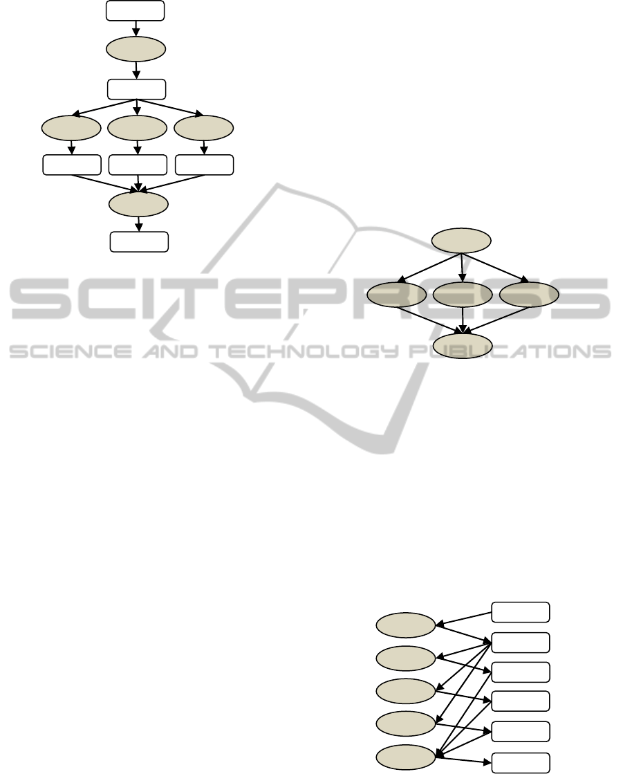
Figure 2: Graphical presentation of workflow in DAG.
3.5 Visualization
Workflow described in our approach can be
visualized as graph of tasks and data. Each task has
directed edges from/to their input/output data. Figure
1 shows the graphical representation of the fork-join
example in Section 3.3 with N=3. In comparison
with the classical DAGs (Figure 2), the graph in
Figure 1 is more informative. If we remove nodes
representing data items by connecting edges to them
with edges from them, the graph in Figure 1 is
identical with the DAG in Figure 2.
Formatteddata
Preprocess
Result[3]
Simulation
Simulation
Simulation
Result[2]
Result[1]
Postprocess
Output
Input
Figure 3: Internal structure of workflow.
It is worth to note that the graph in Figure 1 can
be generated with linear complexity. We don’t have
to analyze every pair of tasks to know if they have
ICSOFT 2011 - 6th International Conference on Software and Data Technologies
232

data dependence, but just read the task description
and make connection to the its data. As every task is
read only once, the complete graph can be generated
with linear complexity. As the graph in Figure 1 is
easily converted to DAG like in Figure 2, we can
prove the statement in Section 3.1 that the workflow
description in our approach can be converted to
DAG with linear complexity.
4 IMPLEMENTATION DETAILS
We use Python scripting language for implementing
a workflow composition tool for processing
workflow description in our approach. With Python,
we can easily write define workflows with loops
and/other control instructions.
Internally, the workflow internally consists of
two lists: list of tasks and list of data. Each task in
the workflow is an object in memory with references
to its data. Figure 3 shows the internal memory
structures of workflows: the list of tasks on the left
side, the list of data on the right side, and references
between tasks and data.
It is interesting to see that the internal data
structure of the workflow in Figure 3 is exactly the
graphical representation of the workflow like in
Figure 1. It means that, once the workflow
description is processed, we have already graphical
representation of the workflow in DAG form in
memory. Therefore, it is easy to export the workflow
description to any other formats compatible with
DAG.
The workflow composition tool can execute the
workflow in three ways:
Execute the workflow locally: The aim of this
mode is for experimentation, verification and
debugging of the composed workflow.
Use other workflow manager as backend: For
executing workflows in Grid, we have implemented
the export of our workflow description to JDL
format.
Use native workflow manager: a native
workflow manager is still in development. It would
exploit the explicit data declaration for performing
direct data transfer among tasks.
5 CONCLUSIONS AND FUTURE
WORK
In this paper, we have presented our approach for
flexible workflow description. Workflows are
described as a list of tasks with input/output data
explicitly defined. This approach supports nested
workflows, loops and other control instructions in
Python scripting language, which is used in our
implementation. The workflows then can be easily
exported to other formats with low complexity.
In the near future, we are developing a
distributed workflow management system natively
based on our approach of workflow description. The
native workflow manager would allow direct data
transfer among tasks according to the input/output
data, without use of storage elements, what would
minimize data transfer and increase performance.
The workflow management system is designed,
implementation is going on.
ACKNOWLEDGEMENTS
This work is supported by projects SMART ITMS:
26240120005, SMART II ITMS: 26240120029,
VEGA 2/0184/10.
REFERENCES
Condor project homepage. http://www.cs.wisc.edu/
condor/. 2011.
D. Hull, K. Wolstencroft, R. Stevens, C. Goble, M.
Pocock, P. Li, and T. Oinn, “Taverna: a tool for
building and running workflows of services” In
Nucleic Acids Research, vol. 34, pp. 729-732, 2006.
E. Laure et al. Programming the Grid with gLite. In
Computational methods in science and technology.
Vol. 12, No. 1, pp. 33-45, 2006.
gLite - Lightweight Middleware for Grid Computing.
http://glite.cern.ch. 2011.
Gregor von Laszewski, Mihael Hategan and Deepti
Kodeboyina. Java CoG Kit Workflow. In Workflows
for E-Science, Part III, pp. 340-356, 2007.
Gregor von Laszewski, Ian Foster, Jarek Gawor, and Peter
Lane. A Java Commodity Grid Kit. In Concurrency
and Computation: Practice and Experience, pp. 643-
662, 2001.
J. Frey. Condor DAGMan: Handling inter-job
dependencies, 2002.
K. Lee, N. W. Paton, R. Sakellariou, E. Deelman, A. A. A.
Fernandes, G. Mehta. Adaptive Workflow Processing
and Execution in Pegasus. In 3rd International
Workshop on Workflow Management and Applications
in Grid Environments, pp. 99-106, 2008.
Kostas Votis et al. Workflow coordination in grid
networks for Supporting enterprise-wide business
Solutions. In IADIS Internacional Conference e-
Commerce, pp. 253-260, 2004.
WORKFLOW COMPOSITION AND DESCRIPTION TOOL
233
