ANALYZING DATA FROM AVL/APC SYSTEM FOR
IMPROVING TRANSIT MANAGEMENT
Theory and Practice
Yun Ye
Nanjing Radio and TV University, No.46, YouFuXi Street, Nanjing, 210002, China
Jie Li
Transportation College, Southeast University, No.2, Sipailou Street, Nanjing, 210096, China
Keywords: AVL, APC transit, Data analysis.
Abstract: AVL (Automatic vehicle location) and APC (Automatic passenger counter) systems are capable of
gathering an enormous quantity and variety of operational, spatial and temporal data that—if captured,
archived, and analyzed properly—hold substantial promise for improving transit performance. Historically,
however, such data has not been used to its full potential. This paper discussed how to use this type of data
to supporting transit service planning, scheduling, and service quality monitoring. First, AVL/APV system
was introduced. Then the actual use and potential uses were reviewed and data requirements for each use
are analyzed. Finally the distribution-based data method was proposed and associated analysis software tool
were developed.
1 INTRODUCTION
The transit industry is in the midst of a revolution
from being data poor to data rich. Traditional
analysis and decision support tools required little
data, not because data has little value, but because
traditional management methods had to
accommodate a scarcity of data. Automatic data
gathering systems do more than meet traditional data
needs; they open the door for new analysis methods
that can be used to improve monitoring, planning,
performance, and management (Furth, 2005).
At first, transit agencies may look to an
automatic data collection system only to provide the
data needed for traditional analyses. But, once they
have the larger and richer data stream that AVL and
APCs offer, they think of new ways to analyze it,
and they want more. Eventually, their whole mode
of operation changes as they become data driven.
This paper proposes a framework for analyzing
AVL and APC data and designed the associated
software tool. It is organized as follow: Section 2
reviews AVL/ APC system to collect data. Section 3
points out the five trends of potential transit data use.
Section 4 describes the analyzing for each use the
kind of AVL-APC data it requires. Section 5 designs
the software tool that facilities analyzing running
time and passenger demand. Section 6 gives the
conclusions.
2 AVL/APC SYSTEM AND DATA
TYPES
2.1 AVL System
In the last decade, global positioning system (GPS)
has become the preferred location technology. GPS
receivers on vehicles determine their location by
triangulation based on signals received from orbiting
satellites. Location accuracy for buses is generally
better than 10 m, depending on the accuracy of
clocks in the GPS receivers and on whether
differential corrections are used.
Because GPS requires a line of sight to the
satellites, GPS signals can be lost as buses pass
through canyons, including man-made canyons
caused by tall buildings. Tall buildings also reflect
267
Ye Y. and Li J..
ANALYZING DATA FROM AVL/APC SYSTEM FOR IMPROVING TRANSIT MANAGEMENT - Theory and Practice.
DOI: 10.5220/0003602402670274
In Proceedings of the 13th International Conference on Enterprise Information Systems (BIS-2011), pages 267-274
ISBN: 978-989-8425-54-6
Copyright
c
 2011 SCITEPRESS (Science and Technology Publications, Lda.)

GPS signals, causing a phenomenon called multipath
that can lead to erroneous location estimation. Older
AVL-APC systems use a combination of beacons,
which serve as fixed-point location devices, and
dead reckoning for determining location between
beacons, using the assumption that the bus is
following a (known) route. All transit coaches have
electronic odometers, making it easy to integrate
odometers into a location system. Route deviations
present a problem for odometer-based dead
reckoning, which is one of the reasons GPS is
preferred. Some AVL systems include a gyroscope,
which makes it possible to track a bus off-route
using dead reckoning. Many GPS-based systems
often use dead reckoning as a backup. When GPS
signals indicate a change in location inconsistent
with the odometer, dead reckoning takes over from
the last reliable GPS measurement, until GPS and
odometer measurements come back into harmony
.Odometers require calibration against known
distances measured using signposts or GPS, because
the relationship between axle rotations (what is
actually measured) and distance covered depends on
changeable factors such as tire inflation and wear.
Therefore，location technologies have been based
on GPS while integrating with other measurements
to improve the accuracy.
2.2 Integrating APC with AVL
Valuable reviews of the history of APCs are found
in reports by Levy and Lawrence (1991), and
Friedman (1993). APCs use a variety of
technologies for counting passengers, including
pressure-sensitive mats, horizontal beams, and
overhead infrared sensing. Automatic passenger
counting has not yet seen widespread adoption
primarily because of its cost and the maintenance
burden it adds. Where adopted, APCs are typically
installed on 10% to 15% of the fleet. Equipped buses
are rotated around the system to provide data on
every route. However, technological advances may
soon make APCs far more common.
The term “APC” can refer to a full data
collection system or to simply the passenger counter
as a device within a larger data collection system.
Historically, APCs were implemented as full,
independent systems that included location
measurement and stop matching. In spite of the
emphasis their name gives to passenger use data,
they not only counted passengers but also provided
valuable operation data that supported analysis of
running time and schedule adherence; in effect, they
doubled as (non-real-time) AVL systems. Canadian
transit agencies have been particularly active in
exploiting APC data.
2.3 Data Type
AVL and APC systems provide four types of data:
2.3.1 Polling Records
Most real-time AVL systems use round-robin
polling to track their vehicles. The polling interval
depends on the number of vehicles being tracked per
radio channel; 40 to 120 s is typical. Within each
polling cycle, every vehicle is polled in turn, and the
vehicle responds with a message in a standard
format. Round-robin polling is an effective protocol
for avoiding message collisions; however, the need
to transmit messages in both directions, with a time
lag at either end for processing and responding,
means that a significant amount of time—on the
order of 0.5 s—is needed to poll each bus. The
polling cycle is therefore limited by the number of
buses being monitored per radio channel. A polling
message includes ID codes (for the vehicle, its run
or block, and perhaps its route) and various fields for
location data. Location fields depend on the location
system used. For a beacon-based system, they
include ID of the most recently passed beacon and
odometer reading.
2.3.2 Event Records
In addition to round-robin polling, WANs also
support messages initiated at the vehicle, generically
called “event messages.” Each event record has a
code and specified format. Modern AVL systems
can have 100 or more different types of event
records. Messages initiated by on-board computers
are likely to collide—that is, one bus will try to send
a message while the channel is busy with another
message. WANs manage this kind of network traffic
problem in various ways, such as by having
messages automatically re-sent until a receipt
message is received. This need to manage traffic
limits the practical capacity of radio-based
communication, because, with randomly arising
messages, the channel has to be unoccupied a
relatively high fraction of the time (unlike with
round-robin polling) to provide an acceptable level
of service. In the face of limited channel capacity,
then, radio-based systems have to be designed in a
way that limits the frequency and length of messages
sent.
ICEIS 2011 - 13th International Conference on Enterprise Information Systems
268

2.3.3 Timepoint Records
In most AVL systems, the timepoint event,
indicating a bus’s arrival or departure from a
timepoint, is the most frequent event record used for
archived data analysis. The event can be defined in
various ways, depending on the location system.
Where GPS is used and door switches are not, it
is common to report when the bus first reaches a
circular zone (typically a 10-m radius) around the
stop. The timepoint record may also include the time
the bus left that zone. In principle, timepoint records
could also include fields indicating when doors first
opened and last closed; however, the researchers are
not aware of any radio-based systems incorporating
door information. The level of detail of timepoint
records affects their accuracy and value for off-line
analysis. For example, some running time and
schedule adherence measures are defined in terms of
departure times, others in terms of arrival times, and
others involve a difference between arrival time at
one point and departure time at a previous timepoint.
Off-line analysis therefore benefits from having both
arrival and departure times recorded, particularly if
operators hold at timepoints. Records of when buses
enter and depart a stop zone are only approximations
of when buses arrive and depart the stop itself.
Errors can be significant in congested areas where
traffic blocks buses from reaching or pulling out of a
stop. Detail on door opening and closing, and on
when the wheels stop and start rolling, can help
resolve ambiguities and make arrival and departure
time determination more accurate.
2.3.4 Stop Records
Stop events are much more frequent than timepoint
events, and therefore, far more demanding of radio
channel capacity if transmitted over the air.
Therefore, most AVL/APC systems collecting data
at the stop-level store stop records in the on-board
computer, uploading them overnight. The data items
typically included in a stop record—in addition to
the usual time stamp, location stamp, vehicle IDs,
and door switches—are door opening and closing
times and (if available) on and off counts. If routes
are tracked by the on-board computer, as is the case
with stop announcement systems, the stop record
will include stop ID in addition to generic location
information; otherwise, the data is matched in later
processing.
3 TRENDS IN DATA USE:
BECOMING DATA RICH
Five trends in data use have emerged from the
paradigm shift from data poor to data rich:
3.1 Focus on Extreme Values
Traditional methods of scheduling and customer
service monitoring generally use mean values of
measured quantities, because mean values can be
estimated using small samples. However, many
management and planning functions are oriented
around extreme values and are, therefore, better
served by direct analysis of extreme values such as
90th- or 95th-percentile values. These extreme
values now can be estimated reliably because of the
large sample sizes afforded by automatic data
collection. Three examples are as follow:
9 Recovery time is put into the schedule to
limit the probability that a bus finishes one
trip so late that its next trip starts late.
Therefore, logically, scheduled half-cycle
times (scheduled running time plus
recovery time) should be based on an
extreme value such as the 95th-percentile
running time. However, without enough
data to estimate the 95th-percentile running
time, traditional practice sets it equal to a
fixed percentage (e.g., 15% or 20%) of
scheduled running time. Yet, some route-
period combinations need more than this
standard, and others less, because they do
not have the same running time variability.
AVL data allows an agency to actually
measure 95th-percentile running times and
use that to set recovery times.
9 Passenger waiting time is an important
measure of service quality. Studies show
that customers are more affected by their
95th-percentile waiting time—for a daily
traveler, roughly the largest amount they
had to wait in the previous month—than
their mean waiting time, because
95thpercentile waiting time is what
passengers have to budget in their travel
plans to be reasonably certain of arriving on
time.
9 Passenger crowding is also a measure in
which extreme values are more important
than mean values. Although traditional
planning uses mean load at the peak point
to set headways and monitor crowding,
ANALYZING DATA FROM AVL/APC SYSTEM FOR IMPROVING TRANSIT MANAGEMENT - Theory and Practice
269

planners understand that what matters for
both passengers and smooth operations is
not mean load but how often buses are
overcrowded. Therefore, design standards
for average peak load are set a considerable
margin below the overcrowding threshold.
However, load variability is not the same on
every route. With a large sample of load
measurements, headways can be designed
and passenger crowding measured based on
90th-percentile loads, or a similar extreme
value, rather than mean loads.
3.2 Customer-oriented Service
Standards and Schedules
AVL-APC data allows customer-oriented service
quality measures to replace (or supplement)
operations-oriented service standards. For example,
on high-frequency routes, a traditional operations-
oriented standard of service quality is the coefficient
of variation (cv) in headway. Although such a
standard may mean something to service analysts, it
means nothing to passengers, and it resists being
given a value to passengers. With a large sample
size of headway data, one can instead measure the
percentage of passengers waiting longer than x
minutes, where x is a threshold of unacceptability.
Similarly, in place of average load factor as a
crowding standard, one could use a standard such as
“no more than 5% of our customers should
experience a bus whose load exceeds x passengers.”
As these examples show, a shift toward customer-
oriented measures goes hand-in-hand with the ability
to measure extreme values.
3.3 Planning for Operational Control
One of the questions posed by the explosion of
information technology is how best to use
information in real time to control operations, for
example, by taking actions such as holding a bus to
protect a connection or having a bus turn back early
or run express. As agencies experiment with, or use,
such actions, they need off-line tools to study the
impacts of these control actions in order to improve
control practices.
For example, AVL-APC data were used to
determine the impacts of a Tri-Met experiment in
which buses were short turned to regularize
headways during the afternoon peak in the
downtown area (Lehtonen, 2002).
3.4 Solutions to Roadway Congestion
Transit agencies are more actively seeking solutions
to traffic congestion, such as signal priority and
various traffic management schemes. They need
tools to monitor whether countermeasures are
effective. In this particular study, only the overall
effect on rather long segments was analyzed by
comparing before and after running times, making
the results hard to correlate with particular
intersections. For better diagnosis and fine-tuning of
countermeasures, agencies need tools to analyze
delays on stop-to-stop, or shorter, segments.
3.5 Discovery of Hidden Trends
Behind a lot of the randomness in transit operations
may be some systematic trends that can be
discovered only with large data samples. For
example, by comparing operators with others
running the same routes in the same periods of the
day, Tri-Met found that much of the observed
variability in running time and schedule deviation is
in fact systematic: some operators are slower and
some faster. Exploratory analysis might also reveal
relationships that can lead to better end-of-line
identification, or to better understanding of terminal
circulation needs.
4 DATA NEEDS FOR SPECIFIC
ANALYSIS
4.1 Running Time
Analyzing and scheduling running time is one of the
richest application areas for archived AVL-APC
data. Without AVL data, agencies must set running
times based on small manual samples, which simply
cannot account for the running time variability that
comes with traffic congestion.
Buses are scheduled at the timepoint level;
therefore, scheduling demands timepoint data.
Because schedules sometimes refer to arrivals as
well as departures, it is helpful if timepoint records
include both arrival and departure times.
Running time analyses that require only
estimation of mean values, or that involve only
occasional studies (e.g., delay and dwell time
analysis), can be conducted with only a sample of
the fleet equipped with AVL. However, routine
scheduling applications based on extreme values
need the entire fleet equipped.
ICEIS 2011 - 13th International Conference on Enterprise Information Systems
270

4.2 Headway Regularity and
Short-headway Waiting
On routes with short headways, headway regularity
is important to passengers because of its impact on
waiting time and crowding. It is also important to
the service provider because crowding tends to slow
operations and because much of operations control is
focused on keeping headways regular.
To measure headways, data has to be captured on
successive trips, making headway analysis
particularly sensitive to the rate of data recovery, as
one lost trip means two lost headways.Analyzing
headway when only part of the bus fleet is
instrumented poses the logistical challenge of
getting all the buses operating on a route to be
instrumented; because of this challenge,
Headways matter all along the route, not only at
timepoints; therefore, stop records are best suited to
headway analysis. (In fact, headways matter most at
stops with high boarding rates.) However, because
headways at neighboring stops are strongly
correlated, timepoints can be thought of as a
representative sample of stops, making it possible,
although not ideal, to estimate headway-related
measures of operational quality from timepoint data.
4.3 Schedule Adherence,
Long-headway Waiting, and
Connection Protection
Monitoring schedule adherence is a valuable
management tool, because good schedule adherence
demands both realistic schedules and good
operational control. It is probably the most common
analysis performed with AVL-APC data. Schedule
adherence can be measured in a summary fashion as
simply the percentage of departures that were in a
defined on-time window, or perhaps as the
percentage that were early, on time, and late.
Standard deviation of schedule deviation is an
indicator of how unpredictable and out of control an
operation is. A distribution of schedule deviations
provides full detail. Such a distribution allows
analysts to vary the “early” and “late” threshold
depending on the application, or to determine the
percentage of trips with different degrees of lateness.
Because schedules are written at the timepoint
level, timepoint data will support schedule
adherence analysis. And because schedule adherence
involves estimating proportions and extremes
(detecting the percentage of early and late trips),the
full fleet should be equipped. Finally, because
schedules sometimes refer to arrival time as well as
departure time, a data collection system that captures
both is preferred.
Passenger waiting time on routes with long
headways is closely related to schedule adherence. It
is possible to determine excess waiting time from
the spread between the 2nd-percentile and 95th-
percentile schedule deviation.
Passengers are particularly interested in whether
they can make their connections. Arriving 4 min late
is not a problem if the time allowed for the transfer
is 5 min, but it could be a big problem if the allowed
time is only 3 min. However, if the departing trip is
held—again, the convergence of schedule planning
and operations control—other issues arise. AVL data
is ideal for determining whether specific connections
were met.
To analyze connection protection an agency must
define the particular connections it wishes to protect
or at least analyze.
Integrating control message data, which might
include requests for holding to help passenger make
a connection, would permit a deeper analysis of
operational control. Incorporating demand data,
ideally transfer volumes, would make the analysis
richer still.
5 RUNNING TIME AND DEMAND
ANALYSIS TOOL
First it is necessary to define the basic input data
collected by AVL/APC, which is served as the basis
for running time and demand analysis.
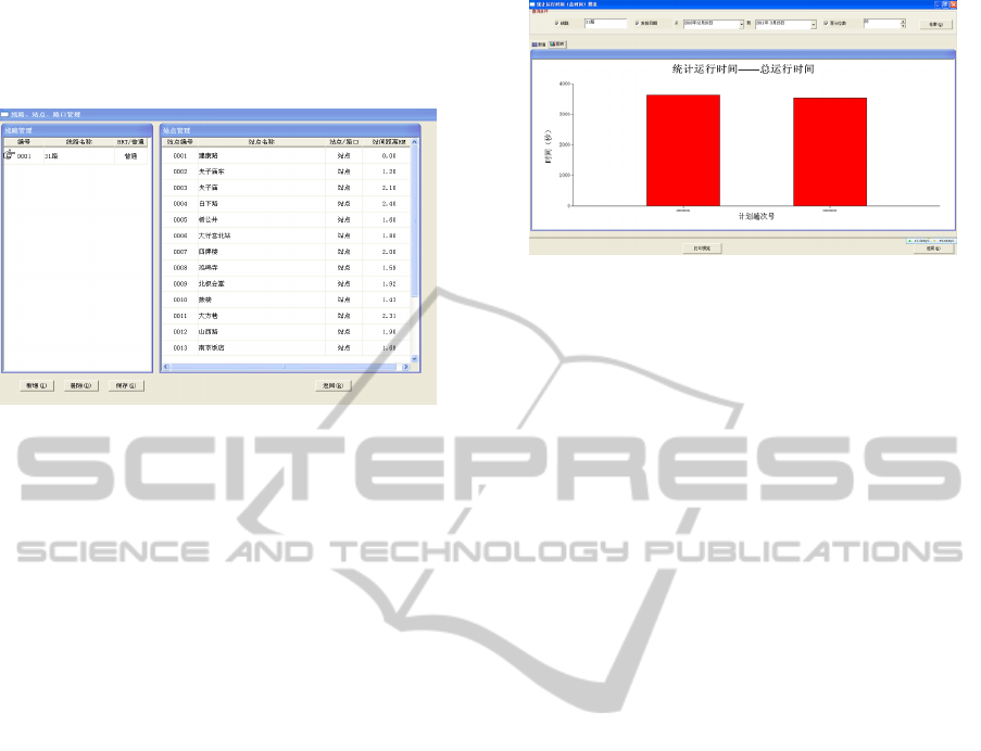
Figure 1: Daily trip records.
Figure 1 shows the basic input data items
including route and trip number, stop name, actual
arrival and departure for each stop for each daily trip,
stop-to-stop distance, etc. Route and stops along it
are created and maintained by a route manger as
shown by Figure 2 .This setting-up facilities input
process and avoid typos by eliminating typing in
these items for each trip. Every time a trip is created,
ANALYZING DATA FROM AVL/APC SYSTEM FOR IMPROVING TRANSIT MANAGEMENT - Theory and Practice
271

only the name or number of the route on which this
trip is made needs to be selected from a drop-down
list. The route manager can update the stop name
and location.
Figure 2: Route and stop manager.
5.1 Scheduled Running Time and
Recovery Time
A common analysis examines the distribution of
observed running time for scheduled trips across the
day. An example is given by Figure 3, the maximum
and minimum observed running time ,mean
observed running time, percentile value for observed
running time was calculated .
Based on the observed distribution of running
time for either a single scheduled trip or a set of
contiguous trips in a period that will be scheduled as
a group, schedule makers can choose a value for
allowed time according to their preferred scheduling
philosophy. Some schedule makers prefer to base
schedules on mean running time. An alternative
approach, aimed at improving schedule adherence, is
to intentionally put slack into the schedule; this
approach has to be coupled with an operating
practice of holding at timepoints. With such a
schedule, a high percentage of trips depart almost
exactly on schedule, and the low percentages of trips
that run late are not far behind schedule. The amount
of slack put into a schedule is often a simple fraction
of mean running time, with ad hoc adjustments
based on experience. A more scientific, data-driven
approach is to use a percentile value, or “feasibility
criterion.” To illustrate, a feasibility criterion of 85%
means setting allowed time (scheduled running time)
equal to 85th-percentile observed running time; such
a schedule can be completed on time 85% of the
time.
Analysis of running time is also pertinent for
determining how much recovery time to schedule at
the end of the line. The time from a bus’s departure
Figure 3: Observed running time distribution for one
single trip.
at one terminal to its next departure in the reverse
direction has been called the “half cycle time”; it is
the sum of running time and recovery time .Because
the purpose of recovery time is to limit the
likelihood that delays encountered in one trip will
propagate to the next, half-cycle time is based
logically on a high-percentile value of running time.
For example, if scheduled recovery time is set to be
the difference between 95th-percentile running times
and allowed time, there will be only a 5% chance
that a bus will arrive so late that it starts the next trip
late.
5.2 Speed and Delay Analysis
Speed, delay, and dwell time studies are analyses
that help support a transit agency’s efforts to
improve commercial speed, something that benefits
both operations and passengers. “Speed” in this
context is average speed over a segment, not
instantaneous or peak speed. A display such as given
in Figure 4 showing delay by segment (or,
alternatively, average speed by segment) helps a
transit agency to identify problem locations, to
monitor the impacts of actions that affect speed, and
to monitor and document historic trends in operating
speed (Barry et al., 2003).
In that figure, it allows analysts to obtain
percentile value of delay, maximum and minimum
delay and mean delay. Analysts will be interested
not only in average delay, but also in how variable it
is, and in the likelihood of extreme values. A report
showing delays or speeds between stops offers a
richer, more geographically detailed view than one
using timepoint segments. Another reason to prefer
stop records as the basis of delay analysis is that it
allows dwell time and control time (which almost
always occur at stops) to be removed, which puts a
clearer focus on the effects of the roadway and
traffic on bus speed and delay.
ICEIS 2011 - 13th International Conference on Enterprise Information Systems
272

Figure 4: Stop-level observed delay distribution.
5.3 Dwell Time Analysis
Transit agencies also try to improve commercial
speed by reducing dwell time, using such measures
as low-floor buses or changes to fare collection
equipment and practices. Stop records with door
open and close times allow agencies to analyze
dwell time to determine impacts and trends. Such an
analysis should preferably be aided by passenger
counts, in order to separate out the impact of the
number of boardings and alightings and to identify
whether any on-vehicle congestion impact arises
when vehicles are crowded. On-off counts, farebox
transactions, and incident codes that reveal
wheelchair and bicycle use are all useful for giving
analysts an understanding of dwell time (Navick and
Fruth, 2002).
Figure 5 shows dwell time distribution for each
stop along a route.
Figure 5.
5.4 Demand Along a Route
The shows not only mean segment loads, but also
mean offs, ons, and through load at each stop in a
single profile. This paper has already pointed out the
importance of extreme values of load for both
passenger service qualities monitoring and
scheduling.
Analysis of demand along a route is necessary
for understanding where along the route high loads
occur. It supports decisions about stop relocation
and installing stop amenities, and routing and
scheduling actions that affect some parts of a route
differently from others, such as short turning, zonal
service, and limited stop service.
Figure 6: Passenger on-off counts and load.
6 CONCLUSIONS
Automatic data collection can revolutionize schedule
planning and operations quality monitoring as
agencies shift from methods constrained by data
scarcity to methods that take advantage of data
abundance. The large sample sizes afforded by
automatic data collection allow analyses that focus
on extreme values, which matter for schedule
planning (e.g., how much running time and recovery
time are needed, what headway is needed to prevent
overloads) and service quality monitoring (e.g., how
long must passengers budget for waiting, how often
do they experience overcrowding). Stop-level data
recording provides a basis for stop-level scheduling,
a practice with potential for improved customer
information and better operational control. With
AVL-APC data, trends can be found that might
otherwise be hidden, such as operator-specific
tendencies and sources of delay en route. Regularly
analyzing AVL data gives a transit agency a tool for
taking greater control of its running times by
offering a means of detecting causes of delay and
evaluating the effectiveness of countermeasures.
REFERENCES
Furth, P. G., J. P. Attanucci, I. Burns, and N. H. Wilson,
2005. Transit Data Collection Design Manual. Report
DOT-I-85-38. U.S.DOT.
Levy, D. and L. Lawrence, 1991. The Use of Automatic
Vehicle Location for Planning and Management
ANALYZING DATA FROM AVL/APC SYSTEM FOR IMPROVING TRANSIT MANAGEMENT - Theory and Practice
273

Information. STRP Report 4, Canadian Urban Transit
Association.
Friedman, T. W.,1993. “The Evolution of Automatic
Passenger Counters.”In Proceedings, Transit Planning
Applications Conference
Navick, D. S. and P. G. Furth, 2002. “Estimating
Passenger Miles, Origin-Destination Patterns, and
Loads with Location-Stamped Farebox
Data.”Transportation Research Record: Journal of the
Transportation Research Board, No. 1799,
Transportation Research Board of the National
Academies, Washington, D.C., 2002, pp. 107–113.
Barry, J. J., R. Newhouser, A. Rahbee, and S. Sayeda.
2003. “Origin and Destination Estimation in New
York City with Automated Fare System Data.”
Transportation Research Record: Journal of the
Transportation Research Board,No. 1817,
Transportation Research Board of the National
Academies, Washington, D.C., , pp. 183–187.
Lehtonen, M. and R. Kulmala. “Benefits of Pilot
Implementation of Public Transport Signal Priorities
and Real-Time Passenger Information.”
Transportation Research Record: Journal of the
Transportation Research Board, No. 1799,
Transportation Research Board of the National
Academies, Washington, D.C., 2002, pp. 18–25.
ICEIS 2011 - 13th International Conference on Enterprise Information Systems
274