
THE EFFECT OF FLUID VISCOSITY IN T-SHAPED
MICROMIXERS
Mina Roudgar, Elizabetta Brunazzi, Chiara Galletti and Roberto Mauri
Department of Chemical Engineering, Industrial Chemistry and Materials Science, University of Pisa
Via Diotisalvi 2, 56126 Pisa, Italy
Keywords: Micromixers, CFD.
Abstract: Effective mixing in small volumes is a crucial step in many chemical and biochemical processes, where
microreactors are to ensure a fast homogenization of the reactants. Physically, liquid flows in microfluidic
channels are characterized by low values of the Reynolds number and, in general, large values of the
massive Peclet number. Accordingly, since general strategies of flow control in microfluidic devices should
not depend on inertial effects, reduction of the mixing length requires that there must be transverse flow
components. In this paper, three-dimensional numerical simulations were performed to study the flow
dynamics and mixing characteristics of liquids flows inside T-shaped micromixers, when the two inlet fluids
are either both water or water and ethanol. In particular we showed that, contrary to what one could think
beforehand, the mixing efficiency of water-ethanol systems is lower than the corresponding water-water
case.
1 INTRODUCTION
Mixing two different fluids in a micromixer is one of
the most basic and revealing case in the general
subject of microfluidics. Due to the small size of the
device, fluids flows are typically laminar, so that, in
simple channels (i.e. with smooth walls), pressure
driven flows are laminar and uniaxial, so that
confluencing liquids tend to flow side by side and
mixing between the two streams is purely diffusive.
To reduce the mixing length, we must induce
transverse flow components that stretch and fold
fluid volumes over the cross section of the channel.
This can be achieved using active or passive
mechanisms (Nguyen and Wu, 2005; Hessel et al.,
2005) .In general, active micro-mixers use external
energy sources, to induce transversal flows and thus
enhance mixing processes, while passive micro-
mixers usually achieve the same effect by using
clever channel geometries to stir or laminate fluids
without external disturbances.The operation of the
passive micromixer is easier and simpler because of
no additional moving parts or energy sources (Yang
and Lin, 2006; Yang et al., 2005; Kim et al., 2004;
Aubin et al., 2005; Wang and Yang, 2006; Wang et
al., 2007).
The simplest designs of a passive micromixers
are T- or Y-shapes. These micromixers are quite
suitable to carry out basic fundamental studies to
understand mixing at the microscale.
Most of the previous works on T- or Y- shape
micromixers is directed towards analyzing mixing
for a wide range of Reynolds numbers and finding
various flow types. It is well known, that the mixing
performance varies significantly with Reynolds
number.
The present study focuses on the effect of the
viscosity difference between the two inlet fluids on
the mixing efficiency in T-type passive micro mixers
for a range of the Reynolds numbers (1 -300). To do
that, a commercial Computational Fluid Dynamic
(CFD) code, FLUENT 6.3 by Ansys Inc., is used to
solve the three-dimensional flow and mass transfer
equations in the proposed geometrical
configurations.
2 SIMULATION TECHNIQUE
2.1 Governing Equations
Consider two fluids converging into a T junction:
the two inlet streams have at the same temperature,
so that, as the heat of mixing has a negligible effect
343
Roudgar M., Brunazzi E., Galletti C. and Mauri R..
THE EFFECT OF FLUID VISCOSITY IN T-SHAPED MICROMIXERS.
DOI: 10.5220/0003601303430347
In Proceedings of 1st International Conference on Simulation and Modeling Methodologies, Technologies and Applications (SIMULTECH-2011), pages
343-347
ISBN: 978-989-8425-78-2
Copyright
c
2011 SCITEPRESS (Science and Technology Publications, Lda.)

here, we may assume that the process is isothermal.
In general, density and viscosity are known
functions of the composition, so that the governing
equations are:
,0=⋅∇+
∂
∂
v
ρ
ρ
t
(1)
()
()
[
]
,gp
ρμρ
+
+
∇+∇⋅∇=∇+∇⋅+ vvvvv
(2)
()
.
2
cDcc ∇=⋅∇+ v
(3)
Here, v denotes the velocity vector, ρ the fluid
density, p the pressure,
μ
the viscosity, g the gravity
acceleration, D the molecular diffusivity (which here
is assumed to be constant) and c the concentration of
one of the two inlet fluids. If the two fluids are
identical, we can imagine adding a very small
amount of contaminant, i.e. a dye, to one of the
fluids (which therefore continue to have the same
physical properties) and therefore c indicates the dye
concentration.
As mentioned in the Introduction, the
characteristics of the velocity and concentration
fields can be described through the Reynolds and
Peclet numbers,
,;
Re
D
Ud
Pe
N
Ud
N ==
ν
(4)
where U is the mean velocity, while the
characteristic fluid length d is assumed to be the
hydraulic diameter D
h
, i.e.,
()
HW
WH
h
Dd
+
==
2
,
(5)
where W and H are the channel width and height,
respectively (see Figure 1).
2.2 Characterization of the Degree
of Mixing
Based on the above considerations, we will use a
definition of mixing efficiency based on material
fluxes, instead of concentration, as the former, not
the letter, are conserved quantities. Accordingly, we
define a cup mixing flow variance as:
dydz
A
cm
cv
zyxczyv
A
x
cm
2
1
),,(),(
1
)(
2
∫
⎥
⎥
⎦
⎤
⎢
⎢
⎣
⎡
−=
σ
i.e.
,
2
1
1
1
2
∑
=
−=
⎟
⎟
⎠
⎞
⎜
⎜
⎝
⎛
N
i
cv
i
c
i
v
N
cm
cm
σ
(6)
where ̅̅
is the (constant) contaminant flux.
For sake of convenience, here we will use the
following definition of degree of mixing,
cmm
σδ
−= 1
(7)
We expect that
δ
m
increases monotonically with x,
tending asymptotically to 1 as the two fluids mix
completely.
2.3 The Inlet Velocity Profile
and the Mixing Zone
The fully developed velocity profile in a closed
rectangular conduit can be easily obtained by
solving the Navier-Stokes equations with no-slip
boundary conditions at the walls and a constant axial
pressure gradient G. For our purposes, the most
convenient form of this solution is (Chatwin and
Sullivan, 1982):
() ()
()
()
()
()
[]
Y
z
kSinh
k
Tanh
Y
z
kCosh
Y
y
k
oddk
k
GY
yYy
G
zyv
π
η
π
ππ
μπ
μ
2
sin
3
1
3
2
4
2
,
−
∑
−−−=
(8)
where Y and Z are the sizes of the conduit, while
η
=Y/Z is the aspect ratio.
From this expression, we can derive the pressure
gradient G as a function of mean velocity
v , finding:
1
2
5
1
5
192
1
2
12
−
∑
−−=
⎥
⎦
⎤
⎢
⎣
⎡
⎟
⎠
⎞
⎜
⎝
⎛
η
π
η
π
μ
k
Tanh
oddk
k
Y
v
G
(9)
We have assumed that the velocity profile
remains fully developed, and therefore given by the
above expression, up to a certain distance from the T
junction, where the influence of vortices and
engulfment of the mixing zone starts to be felt. For
the value of this distance, we used the results given
by Soleymani et al. (2009); who determined it by
numerical simulation.
3 RESULTS AND DISCUSSION
3.1 Numerical Scheme
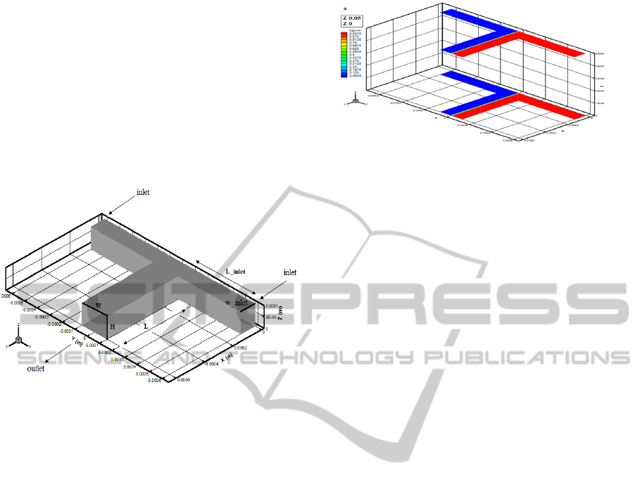
The geometric setting of our simulation, as shown in
Figure 1, is identical to the one used by Bothe
(2006), with two 100
μ
m
×
100
μ
m inlet square
channels and a 200
μ
m
×
100
μ
m mixing channel. The
simulations were conducted using 2.5 μm body-fitted
structured grids in all directions, created by
GAMBIT.
SIMULTECH 2011 - 1st International Conference on Simulation and Modeling Methodologies, Technologies and
Applications
344
At the walls, no-slip and no-mass-flux boundary
conditions were applied, while mass flow rates with
uniform velocity and uniform concentration fields,
were imposed at the entrances. In addition, a
condition of average pressure outlet was set at the
exit of the micromixer. A second order
discretization scheme was used to solve all
equations, using FLUENT 6.3 by Ansys Inc.
Simulation were typically considered converging
when the normalized residuals for velocities fell
below 1× 10
-6
.
Figure 1: Schematics of the T-mixer.
The values of density and viscosity were set
equal to 10
3
kg m
-3
and 10
-3
kg m
-1
s
-1
for water and
789 kg m
-3
and 1.2×10
-3
kg m
-1
s
-1
for ethanol,
respectively , while the diffusion coefficient was set
equal to D = 3.23× 10
-10
m
2
s
-1
, corresponding to
that of a water - ink mixture , as this value is very
close to the self- diffusivity of pure water and of
ethanol as well.
In our simulations, we compared the water-water
case with the water-ethanol case, presenting them
side by side.
3.2 Equal Inlet Velocity
At small flow rates, as wall shear stresses are small,
the two streams behave in the same way, so that the
velocity profile is symmetric along the y-direction
(i.e. along channel width), both near the walls and at
the center of the conduit (see Figure 2 , 3.a and 3.e ).
In fact, at small Reynolds number (Re<30), the flow
patterns in water-water systems is very similar to
those in water-ethanol systems, so that mixing
occurs mainly by mass diffusion and it is therefore
very slow rates with uniform velocity and uniform
concentration fields, were imposed at the entrances.
In addition, a condition of average pressure outlet
was set at the exit of the micromixer.
By increasing the Reynolds number, we see
Figure 2: Mass fraction contour plot at Re = 10 for a
water-ethanol system along the mixing channel close to
the wall and at the channel center.
changes in the flow patterns. In fact, to compensate
for its larger viscosity, ethanol moves slower than
water, so that the pressure drops of the two fluid
streams are equalized. This causes the water moving
to the channel center, while ethanol is driven to the
walls. This phenomenon is more evident when we
move from the channel center to the walls, because
of higher wall shear stresses (see Figure 3.b and 3.f).
Note that the different residence times of the two
fluids does not favor mixing by diffusion in the y-
direction and hence the water-ethanol degree of
mixing in smaller than its water-water counterpart.
At further higher Reynolds numbers, we saw
significant difference in flow patterns and degree of
mixing because of the appearance of the vortices an
engulfment. In fact, as we see in Figure 3.c and 3. d,
in water-water systems, as we move from Re = 100
to Re = 200, we see the appearance of symmetric
vortices and engulfment flows, thus confirming the
results by Bothe (2006). On the other hand, as
shown in Figure 3.g, 3.h and 3.i for water–ethanol
systems the onset of the engulfment regime occurs at
a higher Reynolds number, between. Concomitantly,
in table 1 we see that the two systems exhibit a very
large difference in the degree of mixing δ
m
and wall
shear stresses at the outlet of the micro T-mixer.
3.3 Unequal Inlet Velocity
Our simulation shows that when the two inlet
streams have different velocities (and flow rates as
well), the mixing process is radically different,
depending on whether the majority fluid is water or
ethanol. First, let us consider the behavior of a
water-water system. At low Reynolds number, when
the velocity of the two streams are different from
each other, in Figures 4.a and 4.c we see that, as
expected, the interface moves towards one of the
walls, where the velocity is lower than that at the
centerline (which corresponds to the velocity
experienced by the interface region in the equal
THE EFFECT OF FLUID VISCOSITY IN T-SHAPED MICROMIXERS
345
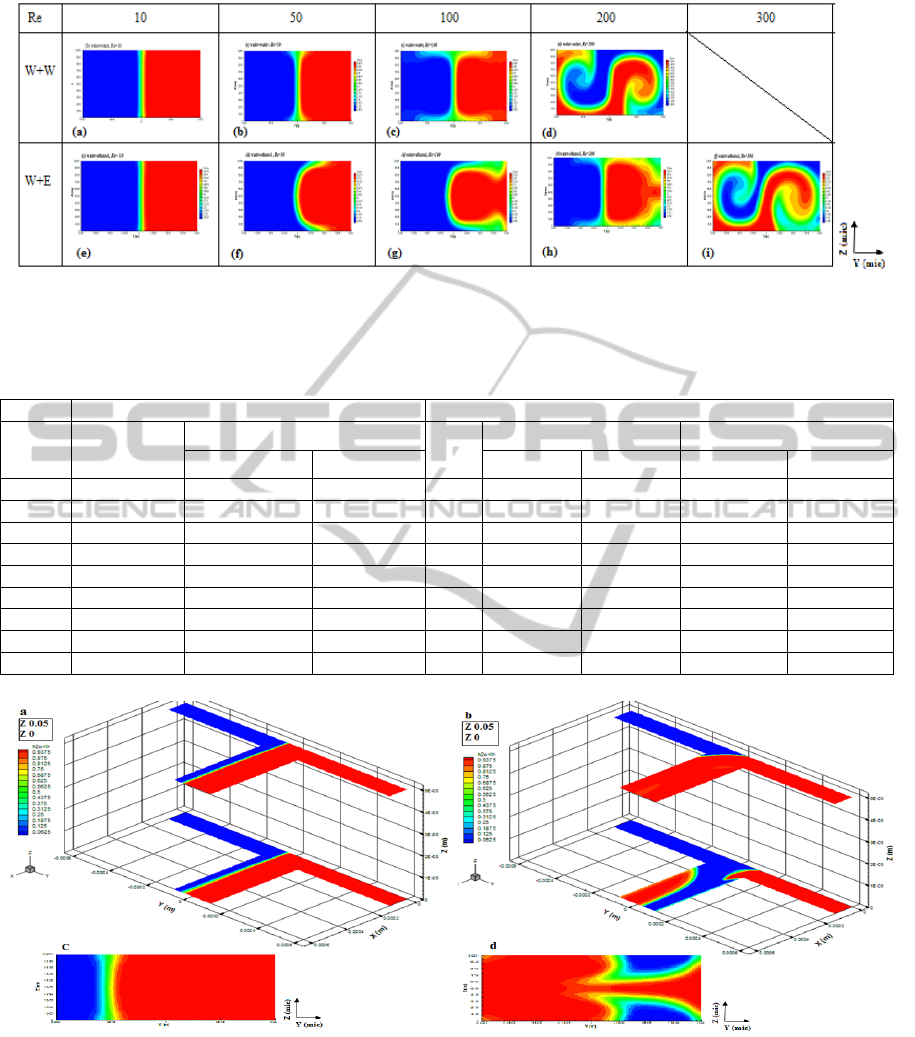
Figure 3: Mass fraction contour plot at different Reynolds number for water-water and b water-ethanol systems at the outlet
cross section.
Table 1: Degree of mixing δ
m
and wall shear stresses at the outlet of the micro T-mixer for water-water and water-ethanol
systems at different Reynolds numbers.
W+W W+E
Re
mix
σ%(mixing
efficiency)
τ(shear stress, mixing)(Pa) σ% τ(inlet channel) τ(mixing channel)
τ
0
(z=0) τ
c
(center) τ
0Water
τ
0Ethanol
τ
0
τ
c
1 4 0.47 0.05 3.2 0.57 0.63 0.514 0.056
10 2 4.7 0.51 1.2 5.31 6.33 5.16 0.57
20 - - - 1.6 10.4 12.7 10 1.1
30 - - - 2 16.3 19.7 15.8 1.66
40 - - - 2.2 22.1 26 21.4 2.2
50 3.6 25 2.5 2.4 28 32.7 27 2.8
100 10 57.4 5.11 5.8 68.5 60 61 5.6
200 26.4 142 12 8.9 133 149 148.4 12
300 41 31 218 235 248 21
Figure 4: Mass fraction contour plots of water-water systems at a velocity ratio V
1
/V
2
=
β
=5 along the mixing channel
(close to the wall and at the channel center) and at the outlet cross section for a) and c) Re = 1; c) and d) Re = 100 .
velocity case). Accordingly, as the diffusion time is
larger than that in the equal velocity case, the mixing
degree increases also. Then, at larger Reynolds
numbers, in Figures 4.b and 4.d we see that the
faster fluid stream hops to the opposite side of the
mixing channel, leaving the slower fluid close to the
walls, resulting in an increase of a mixing efficiency.
In water-ethanol systems, when the water stream is
faster, we observe a behavior that is very similar to
that of water-water systems, although, as shown in
Table 2, the degree of mixing is smaller.
SIMULTECH 2011 - 1st International Conference on Simulation and Modeling Methodologies, Technologies and
Applications
346
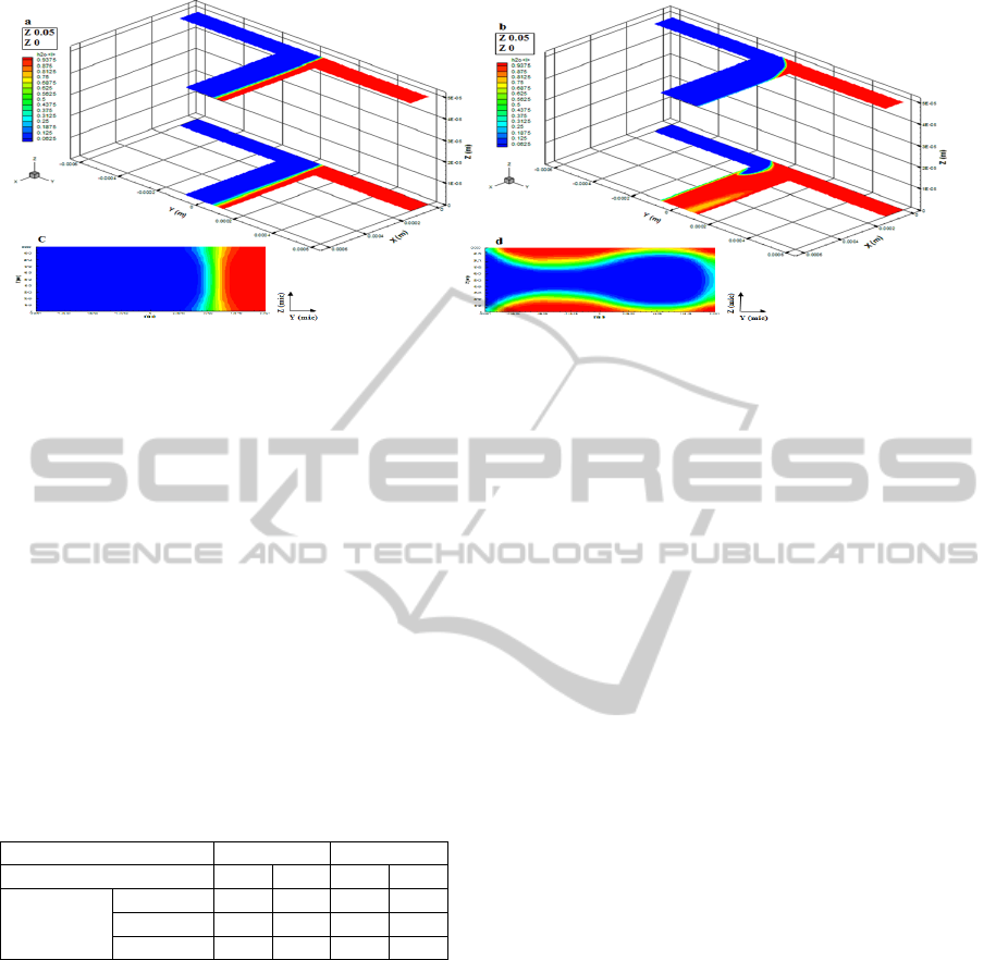
Figure 5: Mass fraction contour plots of water-ethanol systems at a velocity ratio V
e
/V
w
=
β
=5 along the mixing channel
(close to the wall and at the channel center) and at the outlet cross section for a) and c) Re = 1; c) and d) Re = 100 .
On the other hand, for water-ethanol systems
with ethanol being the faster stream, the behavior is
radically different, as shown in Figure 7. In fact, in
this case, comparing Fig. 4.d with 5.d, we see that at
high Reynolds number, the faster stream, i.e.
ethanol, now tends to hop to the opposite side even
more easily, generating a phase pattern that is quite
different. In addition, at low Reynolds number,
comparing 4.c with 5.c, we see that the interface
region is thicker and therefore the degree of mixing
is higher. These observations are summarized in
Table 2.
Table 2: Degree of mixing δ
m
at the outlet of the micro T-
mixer for water-water and water-ethanol systems at
different Reynolds numbers and inlet velocity ratios.
Systems W+W W+E
Re 1 100 1 100
σ%(mixing
efficiency)
V1/V2=5 9.5 28 - -
Vw/Ve=5 - - 5.7 23
Ve/Vw=5 - - 15.8 27
4 CONCLUSIONS
Three-dimensional numerical simulations were
performed to study the flow dynamics and mixing
characteristics of liquids flows inside T-shaped
micromixers, when the two inlet fluids are either
both water or water and ethanol. In particular we
showed that, predictably, the degree of mixing is
larger for unequal inlet flow rates. On the other
hand, contrary to what one could think beforehand,
the mixing efficiency of water-ethanol systems is
lower than the corresponding water-water case.
REFERENCES
Nguyen, N. T., & Wu, Z. G., (2005). Micromixers-a
review. Journal of Micromechanics and
Microengineering, 15, R1–R16.
Hessel, V., Lowe, H., Schonfeld, F. (2005). Micromixers-a
review on passive and active mixing principles.
Chemical Engineering Science, 60, 2479– 2501.
Yang, J. T., & Lin, K. W. (2006). Mixing and separation
of two-fluid flow in a micro planar serpentine channel.
Journal of Micromechanics and Microengineering,
16, 2439–2448.
Yang, J. T., Huang, K. J., Lin, Y. C. (2005). Geometric
effects on fluid mixing in passive grooved
micromixers. Lab on a Chip, 5, 1140–1147.
Kim, D. S., Lee, S. W., Kwon, T. H., Lee, S. S. (2004). A
barrier-embedded chaotic micromixer. Journal of
Micromechanics and Microengineering ,14, 798–805.
Aubin, J., Fletcher, D. F., Xuereb, C. (2005). Design of
micromixers using CFD modeling. Chemical
Engineering Science, 60, 2503–2516.
Wang, L., & Yang, J. T. (2006) An overlapping crisscross
micromixer using chaotic mixing principles. Journal
of Micromechanics and Microengineering, 16, 2684–2691.
Wang, L., Yang, J. T., Lyu, P. C. (2007). An overlapping
crisscross micromixer. Chemical Engineering Science,
62, 711–720.
Chatwin, P. C. & Sullivan, P. J. (1982). The effect of
aspect ratio on the longitudinal diffusivity in
rectangular channels. Journal of Fluid Mechanic, 120,
347-358.
Bothe, D., Sternich, C., Warnecke, H. J. (2006). Fluid
mixing in a T-shaped micro-mixer. Chemical
Engineering Science, 61, 2950–2958.
Lee, S., Lee, H. Y., Lee, I. F., Tseng, C.Y. (2004). Ink
diffusion in water. European Journal of Physics, 25,
331–336.
Soleymani, A., Yousefi. H., Ratchananusorn, W.,
Turunen, I. (2010). Pressure drop in micro T-mixers.
Journal of Micromechanics and Microengineering, 20,
015-029.
THE EFFECT OF FLUID VISCOSITY IN T-SHAPED MICROMIXERS
347
