
THE RESEARCH ON STABILITY OF SUPPLY CHAIN UNDER
HIGH ORDER DELAY
Jia Su-ling, Wang Lin, Luo Chang and Wang Qiang
School of Economics & Management, Beihang University, XueYuan Road No.37, HaiDian District, Beijing, China
Keywords: Supply chain, Stability, High order delay, Simulation, System dynamics.
Abstract: Based on system dynamics (SD), a high order delay inventory control model of supply chain is proposed. The
high order delay in SD is regarded as transition between first order lag and pure time delay (PTD), it describes
the more general delay mode in real systems. With simulation, the stable boundaries of inventory control
model under high order delay are confirmed, and the effect of variations in delay mode on stability of
inventory control system is analyzed. It is concluded that the reduction of delay order and delay time can
improve the stability of inventory control model under high order delay; the sensibility of decision parameters
to the change of system order is nonlinear.
1 INTRODUCTION
Bullwhip effect have triggered a series of problems
including the increase of the operational risk of
enterprise and the decline in supply chain
management efficiency (Lee et al., 1997).In recent
years, the dynamic characteristic of supply chain
represented by bullwhip effect had received
considerable attention. The research on stability of
supply chain is helpful to reduce the bullwhip effect
and improve the operation benefit of supply chain.
In the research of stability of supply chain, the
delay structure is a key influencing factor of system
stability. The researches based on the hypothesis of
first order lag focused on revealing the influence of
management practices to the fluctuant phenomenon
in supply chain and proposed several management
strategies to eliminate the bullwhip effect
(Balakrishnan et al., 2004; Disney et al., 2004;
ChengHu et al., 2005; Zhang et al., 2006). Riddalls et
al. (2000) first pointed out that there was difference
between first order models and actual systems.
Henceforth, the studies based on pure time delay
(PTD) emphasized that supply chain structure
determined the convergence of inventory and order
(Riddalls and Bennett, 2002; Warburton, 2004;
Huixin and Hongwei, 2004). Under the influence of
many factors, the delay mode of the actual inventory
control system may be the high order delay which is
the mixed form of first order lag and pure time delay.
As system dynamics (SD) has provided the
scientific basis for describing high order delay
structure, it avoids the obstacle of analytic modeling
in this area. In this paper, we adopt high order delay as
the transition between first-order delay and pure time
delay and built the supply chain SD model. Through
simulation, the dynamic characteristics and stability
of the system are analyzed.
2 HIGH ORDER DELAY
INVENTORY CONTROL
SYSTEM MODEL
2.1 The Implication of High Order
Delay
In a stable production or transportation system, there
exists an average delay time and the distribution of
output with delay is stable. In system dynamics, the
distribution is described by high order delay.
First order delay and pure time delay are the
particular cases of high order delay. System
dynamics suggests that the structure of first order
delay is equivalent to the structure of negative
feedback with linear first-order, and the structure of
high order delay is equivalent to several first-order
delaying links connected in series. When the order of
high order delay approaches to infinity, high order
361
Su-ling J., Lin W., Chang L. and Qiang W..
THE RESEARCH ON STABILITY OF SUPPLY CHAIN UNDER HIGH ORDER DELAY.
DOI: 10.5220/0003583103610367
In Proceedings of the 13th International Conference on Enterprise Information Systems (SSSCM-2011), pages 361-367
ISBN: 978-989-8425-54-6
Copyright
c
2011 SCITEPRESS (Science and Technology Publications, Lda.)
delay is equivalent to pure time delay (Riddalls and
Bennett , 2002).
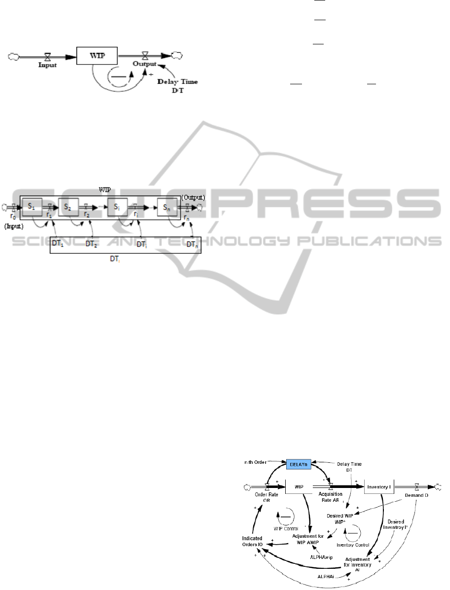
The structure of linear first-order system with
negative feedback is shown as follows:
Figure 1: Structure of linear first-order system with
negative feedback.
Output is described as:
Output (t) = WIP/DT (1)
Connecting n first-order delaying links in series,
we can obtain the n orders delay:
Figure 2: Structure of high order delay.
The notation for the model presented in figure 2 is as
follows:
r
i
: input (output) flow at the middle levels. r
0
and r
n
are the input and output of the
model. i = 0,1,…, n
S
i
: the delayed flow at the middle levels, i =
1,2,…, n
WIP:the total flow
DT
i
: the delay time at the middle levels, i =
1,2,…, n
DT:the total delay time
The relationship between the total flow and the
delayed flow at the middle levels is:
WIP=
∑
S
(2)
The total delay time and the delay time at the
middle levels can be simplified (Sterman J. D, 2000):
DT=
∑
DT
DT
=DT
=⋯=DT
=DT/n
(3)
Refer to the structure of first order delay, the
relationship between the input and output at the
middle levels can be represented by differential
equations:
r
=
n
DT
(r
−r
)
r
=
n
DT
(r
−r
)
…
r
=
n
DT
(r
−r
)
(4)
That is:
r
−DTr
′
+
r
′′
+⋯+
(
−1
)
(
)
r
()
=r
(5)
Eq. (5) indicates that it is very difficult to
calculate the output flow r
n
and the delayed flow at
the middle levels may be not differentiable in real
system. Through the analysis of the structure of high
order delay shown in figure 2, we can find that the
greater the order n, the smaller the delay time at the
middle levels DT
i
will be. When the order n
approaches infinity, DT/n is equal to DT
i
and both
are close to zero. That is:
r
0
≈r
1
≈r
2
≈…≈r
i
≈…≈r
n
(6)
r
n
≈r
0
(t - DT) (7)
Therefore, pure time delay can be approximated
by limited high order delay, and the smaller the DT
i
,
the higher the degree of approximation is. It also
indicates that high order delay is the smooth
transition between first order delay and pure time
delay.
System dynamics simulation software, Vensim
PLE, has provided the function of high order delay:
DELAY
n
(Input, Delay Time, n)
Where n is the order of high order delay.
2.2 Model Structure
Figure 3 shows the high order delay inventory control
model of supply chain that is built on the basis of the
generic stock-management model proposed by
Sterman (1989).
Considering that the validity of demand forecasting
will influence the system stability, we
Figure 3: High order delay inventory control model.
ICEIS 2011 - 13th International Conference on Enterprise Information Systems
362
do not make prediction on market demand. The
adjustments include two aspects:
DELAY
n
: the limited high order delay mode of
WIP;
n-th Order: delay parameter, the order of high
order delay.
In the model, the decision maker first
determines the desired WIP based on demand and
delay time, and then determines the actual
adjustment for WIP. Finally, the order to upstream
will be made according to demand and adjustment
for inventory and WIP.
The expression of the relationship between
order rate and acquisition rate is as follows:
AR = DELAY
n
(OR, DT, n-th Order)
Table 1 shows the variable settings (Sterman,
1989).
Where α
i
is the rate at which the discrepancy
between actual and desired inventory levels is
eliminated, and α
WIP
is the rate at which the
discrepancy between actual and desired WIP levels is
eliminated, 0≤α
i
, α
WIP
≤1. The values of α
i
and α
WIP
represent the sensitivity of decision-maker to the gaps,
that is, (I*-I) and (WIP*-WIP).
Table 1: Variable settings.
Variable Expression
WIP
I
AR DELAY(OR, DT)
AI α
i
(I
*
- I)
AWIP α
WIP
(WIP
*
- WIP)
IO D + AI + AWIP
OR Max(0, IO)
ALPHAi 0≤α
i
≤1
ALPHAwip 0≤α
WIP
≤1
3 STABILITY ANALYSIS AND
CRITERIA OF SUPPLY CHAIN
3.1 The Definition of Stability
There are different definitions of stability of supply
chain. The traditional ideas of system dynamics state
that only the behavior of smooth convergence is
stable while the other fluctuate behaviors are unstable
(Forrester, 1958). The main reason is that system
dynamics methods focus on systems under first order
lag. Scholars based on control theory stress the
importance of pure time delay, it is commonly
accepted that fluctuant convergence is a gradual
process of system to be stable and oscillation with
equi-amplitude is a critical state of stable system.
Based on the definition of stability in control theory
and the methods applied by system dynamics, we
propose the following definition of stability of supply
chain system:
Definition 2.1: Suppose the system is stable at
the initial time, when imposing a small step
disturbance on demand, if the inventory (or order rate)
can get stable at a certain equilibrium level after a
period of time, then the system is stable.
3.2 Stability Criterion
Combining with the above definition of stability, this
paper takes inventory as research subject to obtain
the stability criterion. As the underlying cause of the
fluctuation of inventory is the deviation between
actual inventory and desired inventory, we use the
area between the two curves to describe the
fluctuation in supply chain. This practice is similar
to the method in cybernetics that use “noise
bandwidth” to make quantitative description of
bullwhip effect (Dejonckheere , 2003; Wang et al.,
2006).
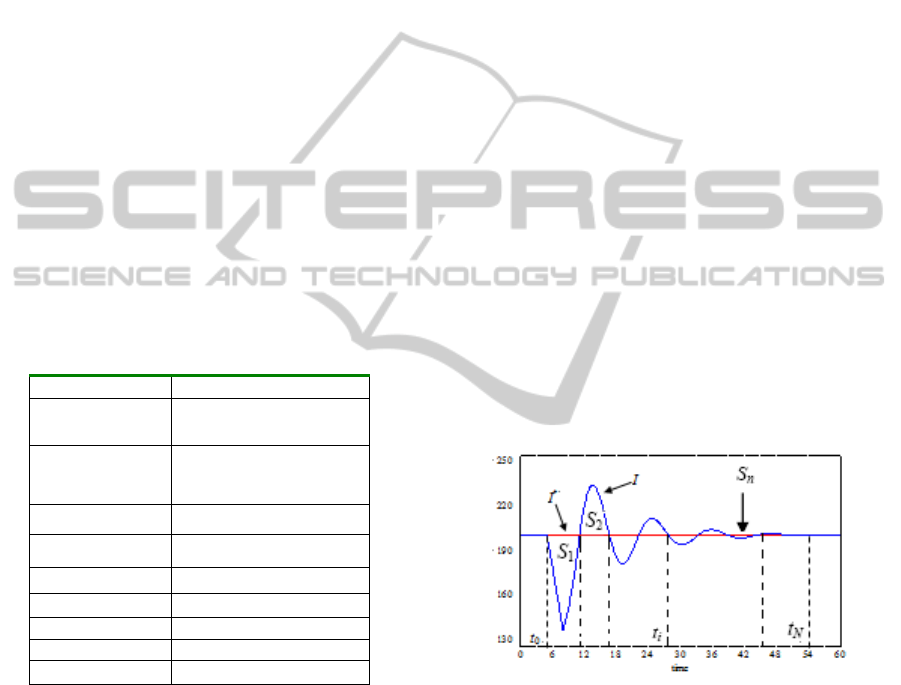
Figure 4 shows the general behavior pattern of
inventory fluctuation.
Figure 4: General behavior pattern of inventory
fluctuation.
As shown in figure 4, assuming that the
inventory curve begins to fluctuate at time t
0
, the
inventory curve and desired inventory level intersect
at time t
1
, t
2
…t
i
…t
n
in succession, and the area
between two curves can be divided into several parts
S
1
,S
2
…S
i
...S
n
. Let the absolute value of the area
between the two curves be s
n
,that is:
S=
∑|
S
|
=
|
I
(
t
)
−I
∗
|
dt
(8)
We can distinguish the behavior of the system
according to the form of curve S, that is, S curve can
0
0
[() ()]
t
t
t
OR t AR t dt WIP
∫
0
0
[() ()]
t
t
t
AR t D t dt I
∫
THE RESEARCH ON STABILITY OF SUPPLY CHAIN UNDER HIGH ORDER DELAY
363
be used as the stability criterion of the system and it
can be obtained by the software, Vensim PLE.
According to the definition of stability, the
sufficient condition of the system to be stable is
presented as following:
lim
→∞
S(t)=C (Constant) (9)
Eq. (9) can be replaced by the following
description:
Assuming t
0
is the starting time of simulation
and t
F
is the end time of simulation, if there exists t
s
(t
0
≤t
s
≤t
F
) to make S(t) = C (Constant), then the system
is stable.
The constant C can be understood as the system
stable level, and the smaller the value of C, the better
stability of the system. In the condition of step
disturbances on demand and no prediction, C is
positive.
4 STABILITY ANALYSIS OF
HIGH ORDER DELAY
INVENTORY CONTROL
SYSTEM
4.1 Simulation Design
The initial values (unit) of variables are presented in
Table 2 (Sterman, 1989; Riddalls and Bennett, 2002).
The model is built using well-known system
dynamics simulation software, Vensim PLE. The run
length for simulation is 60 weeks.
Table 2: Initial Conditions.
I
*
DT α
i
α
WIP
n
MAX
Step
300 200 200 3 1 0 100 50 0.0625
We adopt the small disturbance on demand for
stability examination. This method has been widely
used in the study of system stability based on control
theory and general system theory. The order of delay
gradually increases from 1 to n
MAX
and the demand
function is as follows:
D=D
t0
(1+STEP(h,T
s
)) (10)
Where h is the step signal of amplitude and Ts is
the moment when step change happens. h = 0.2,Ts =
5.
In the presence of small disturbance, the
decision parameter α
i
is changed from 1 to 0 with a
small decrement Δi. At the same time, α
WIP
varies
from 0 to 1 with another small increment ΔWIP, the
smaller the values of Δi and ΔWIP, the higher the
simulation accuracy. Meanwhile, the order of delay
gradually increases from 1 to n
MAX
.
Through simulation, we can observe the
behavior patterns of the high order delay inventory
control model and test the system stability in the
situation of complete rationality (α
i,
α
WIP
∈
[0,1]).
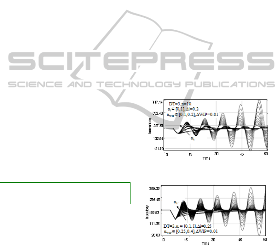
4.2 Dynamics Characteristics
Figure 5 and figure 6 have shown the traverse graphs
of inventory curves of tenth-order delay system and
PTD system. Simulations indicate that the behavior
patterns of inventory shown in figure 5 can represent
the general dynamics characteristics of high order
delay system. It is concluded that high order delay
system can be presence of oscillation with
equi-amplitude and divergent fluctuation, and the
parameters α
WIP
and α
i
show entirely opposite effects
on the dynamics characteristics of high order delay
system. Based on the analysis, we can conclude that
high order delay system has stability boundary
corresponding to PTD system.
Figure 5: The traverse graph of inventory curves of
tenth-order delay system.
Figure 6: The traverse graph of inventory curves of PTD
system.
4.3 Stability Analysis
As high order delay system covers four kinds of
behavior patterns: smooth convergence, fluctuant
convergence, oscillation with equi-amplitude,
divergent fluctuation, it is more appropriate to PTD
0
t
WIP
0
t
I
0
t
D
ICEIS 2011 - 13th International Conference on Enterprise Information Systems
364
system from the visual point of view. The contrast
between figure 5 and figure 6 shows that the range of
decision parameter α
WIP
in ninth-order delay system
is smaller than that in PTD system with the same
delay time and range of decision parameter α
i
. That
is, in high order delay system, the decision maker
can consider more about inventory and consider less
about WIP. Beer game has shown that most
decision-makers think that the actual inventory is
more important than WIP. Therefore, even if the
decision maker has bias against the above conclusion,
the high order delay system may still be stable. In
other words, the decision strategies that lead PTD
system to be unstable may make high order delay
system stable. So, high order delay system is more
stable than PTD system.
Through simulations, we can find the critical
stable state of n-th order delay system with a given
DT and obtain the critical stable points (α
,
, α
,
).
Therefore, the critical stable condition of inventory
control system under n-th order delay is defined as
following:
Definition: Suppose the n-th order delay
inventory control system is stable at the initial time.
With a given DT, when imposing a small step
disturbance on demand, if there exists the decision
parameters (α
,
, α
,
) that can keep the inventory
curve oscillate with equi-amplitude, then the state is
called critical stable state, (α
,
, α
,
) is the critical
stable point of the system under the given DT.
As high order delay system considers the order of
delay, its critical stable points are determined by four
dimensional vectors, (DT, α
i
, α
WIP
, n). Through the
traversal simulation of α
i
and α
WIP
under certain DT,
several critical stable points are found. After
connecting these points in the plane that takes α
i
as
horizontal axis and α
WIP
as vertical axis, we obtain
the stability boundary of the tenth-order delay
system named s curve. Figure 7 shows some s curves
under different DT and the index of s represents the
value of DT. For comparison, the corresponding
stability boundaries of PTD system are also given.
Figure 7: Comparison between the stability boundaries of
tenth-order delay system and PTD system.
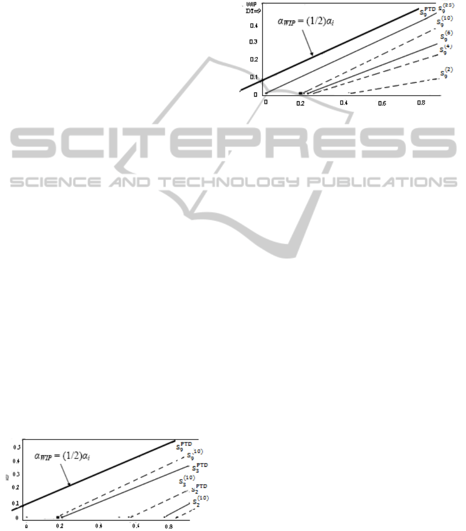
Furthermore, s curve of high order delay system is
approximate to linear property and the lower right of
s curve is the unstable region. For comparison, figure
8 shows the stability boundaries of five high order
delay systems with different delay orders
(n=2,4,6,10,25) under certain DT (DT=9).
Figure 8: The effect of delay order on system stability
(DT=9).
After running simulations for the high order
delay inventory control model under different DT
and comparing with PTD system, we can draw the
following conclusions:
First, the stable region of high order delay
system is larger than that of PTD system. With the
same delay time, the larger order of delay, the closer
the stability behavior of high order delay system to
PTD system, and the oblique line (α
WIP
=α
i
/2) is the
upper bound when s curve moves up to top left.
Second, as the oblique line (α
WIP
=α
i
/2) is the
upper bound when s curve of n-th order delay
inventory control system moves up to top left with
certain DT, it can be concluded that the upper left
area of oblique line (α
WIP
=α
i
/2) is the stable region
which is independent of delay (IoD), and the oblique
line (α
WIP
=α
i
/2) can be defined as IoD stability
boundary which is only determined by systemic
structure.
Third, under the same delay condition, the
smaller delay time, the larger the stable region of
high order delay time; and under the same delay time,
the smaller the order of delay, the larger the stable
region. Therefore, the stability of high order delay
system with short delay time and small order of
delay is closer to first-order system.
Further analysis on figure 8 reveals that when
the order of delay is small, the s curves tend to be
relative dispersive, and when the order of delay is
large, the s curves are comparatively concentrated.
This shows that the sensibility of decision
parameters to the change of system order is
nonlinear.
Based on figure 8, when the decision parameter
α
i
takes a certain value, figure 9 shows the relation
THE RESEARCH ON STABILITY OF SUPPLY CHAIN UNDER HIGH ORDER DELAY
365
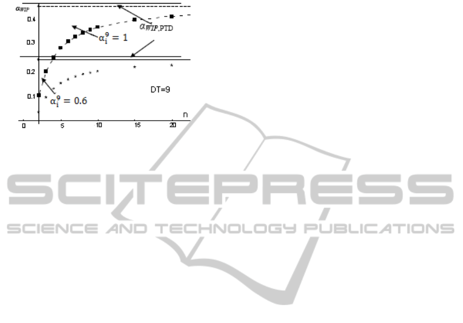
curves between the decision parameter α
WIP
and the
order of delay (
α
i
=0.6; α
i
=1).
Figure 9: The delay order's sensitivity curve.
Figure 9 indicates that under the given delay time
and decision parameter α
i
, the value of α
WIP
increases
as the order of delay increases and it finally tends to
that of PTD system in the same condition, but the
increase margin of α
WIP
drops when the order of
delay increases. In other words, when the order of
delay is large, the decision parameter α
WIP
has a low
sensitivity to the change of it. After simulations of
delay systems under different DT, the above
nonlinear characteristics still exist in the system.
The analysis above shows that in order to
maintain system stability, decision maker should
make clear the delay mode of WIP when focusing on
the change of inventory and WIP. Overestimating
the order of delay will artificially limit the stable
region and restrict the implementation of certain
ordering strategies. At the same time,
underestimating the order of delay may enlarge the
stable region and result in accidental fluctuations in
the system.
4.4 Discussion
The structure of high order delay is the transition
between first-order delay and pure time delay and it
describes the more general delay mode in real
systems. Therefore, it is more accurate to assume the
delay mode in real systems to be high order delay.
Researchers have shown that the delay mode of WIP
is determined by the service rules of system and the
order of delay is an important parameter to describe
the delay mode. The order of delay can be
approximately evaluated based on system data and
then be used for simulation.
Simulation results show that system stability
can be improved through decreasing the order of
delay and shortening the delay time. Decreasing the
order of delay suggests the adjustment on service
rules, that is, the production or transportation system
must be designed reasonablely. So decreasing the
order of delay system can improve both the system
stability and the overall level of service.
Finally, although the stability boundary of
system exists objectively, it is definitely difficult to
obtain the stability boundaries from theory or
simulation. The inaccurate estimate of decision
maker on the delay mode will lead to wrong decision
and even the optimized rules may make the system
instable. Therefore, to strengthen the control to the
system and avoid the subjective error are important
means of increasing system stability.
5 CONCLUSIONS
To conduct quantitative analysis on the stability of
high order delay system, we first give the abstract
analysis on the structure of high order delay and then
built the high order delay inventory control model of
supply chain. By simulation analysis, a
system-dynamics-based criterion for stability
judgment is proposed. With simulation, the criterion
can be used to describe the nonlinearities of supply
chain system and judge the influences exerted on
supply chain stability by decision behavior.
According to the concept of stability and stability
criterion proposed in the paper, stability boundaries of
high order delay inventory control system are
confirmed. It is concluded that the IoD stability
boundary has nothing to do with the delay time and
order of delay and the stability of high order delay
inventory control system is mainly decided by the
features of feedback systems.
As high order delay system considers the order
of delay, this paper further analyzes the effect of
order of delay on system stability and finds that the
sensibility of decision parameters to the change of
system order is nonlinear. Synthetic analysis indicates
that the subjective sensation of decision maker on the
structure and behavioral pattern of system has great
influence on the system stability. The paper finally
points out that system stability and the overall level of
service can be improved by adjusting the service rules
in inventory control system, and further research
needs to be done on how to adjust the service rules.
REFERENCES
Lee H. L., Padmanabhan V., Whang S.(1997). The bullwhip
effect in supply chains. Sloan Management Review,
38(3), 93–102.
ICEIS 2011 - 13th International Conference on Enterprise Information Systems
366

Balakrishnan A, Geunes J, Pangburn M.S. (2004).
Coordinating supply chains by controlling upstream
variability propagation. Manufacturing and Service
Operations Management, 6, 163–183.
Disney S. M., Towill D. R., Van De Velde W.
(2004).Variance amplification and the golden ratio in
production and inventory control. International Journal
of Production Economics, 90(3), 295-309.
Chen Hu, Han Yuqi, Wang Bin, (2005). The Study of
Inventory Management Based on System Dynamics.
Journal of Industrial Engineering and Engineering
Management. 19(3), 132-140.
Zhang Libo, Han Yuqi, Chen Jie et al. (2006). System
Dynamics in Plant Capacity Enlargement. Journal of
System Simulation. 18(5), 1327-1330.
Riddalls C. E., Bennett S, Tipi N.S. (2000). Modeling the
dynamics of supply chains. International Journal of
System Science, 31(8), 969-976.
Riddalls C. E., Bennett S. (2002). Production-inventory
system controller design and supply chain dynamics.
International Journal of Systems Science, 33(3),
181-195.
Warburton R. D. H. (2004). An exact analytical solution to
the production inventory control problem. International
Journal of Production Economics.92 (1), 81-96.
Liu Huixin, Wang Hongwei. (2004). Performance analysis
of a supply chain under order-up-to policy. Computer
Integrated Manufacturing Systems, 10(8), 939-944.
Riddalls C. E., Bennett S. (2002).The stability of supply
chains. International Journal of Production Research,
40,459-475.
Sterman J. D. (2000). Business Dynamics: Systems
Thinking and Modeling for a Complex World. New
York: McGraw –Hill /Irwin.
Sterman J D. (1989). Modeling managerial behavior:
misperceptions of feedback in a dynamic
decision-making experiment. Management Science,
35(3):, 321-339.
Forrester J. W. 1958.Industrial dynamics: a major
breakthrough for decision makers. Harvard Business
Review. 36(4): 37–66.
Dejonckheere J., Disney S. M., Lambrecht, M. R. et al.
(2003).Measuring and avoiding the bullwhip effect: A
control theoretic approach. European Journal of
Operational Research, 147(3), 567-590.
Wang Jing, Sun Haiyan, Li Yilan, (2006).Irregular
information distortion and weakening methods in
supply chains. Journal of Beijing University of
Aeronautics and Astronautics.32 (12), 1481-1484.
THE RESEARCH ON STABILITY OF SUPPLY CHAIN UNDER HIGH ORDER DELAY
367
