SIMULATION OF NONLINEAR DIFFUSION ON A SPHERE
Yuri N. Skiba
Centre for Atmospheric Sciences (CCA), National Autonomous University of Mexico (UNAM)
Av. Universidad 3000, C.P. 04510, Mexico City, Mexico
Denis M. Filatov
Centre for Computing Research (CIC), National Polytechnic Institute (IPN)
Av. Juan de Dios Batiz s/n, C.P. 07738, Mexico City, Mexico
Keywords:
Simulation of environmental problems, Nonlinear diffusion, Split finite difference schemes.
Abstract:
A new numerical technique for the simulation of nonlinear diffusion processes on a sphere is developed. The
core of our approach is to split the original equation’s operator, thus reducing the two-dimensional problem to
two one-dimentional problems. Further, we apply two different coordinate grids to cover the entire sphere for
solving the split 1D problems. This allows avoiding the question of imposing adequate boundary conditions
near the poles, which is always a serious problem when modelling on a sphere. Yet, therefore we can employ
finite difference schemes of any even approximation order in space. The developed approach is cheap to
implement from the computational point of view. Numerical experiments prove the suggested technique,
simulating several diffusion phenomena with high accuracy.
1 INTRODUCTION
A large number of important natural phenomena, e.g.,
heat transfer in ionised gases, unconfined groundwa-
ter flow and gas percolation through porous media,
viscous liquid flows over smooth horizontal substrates
— just to name a few — are described by nonlinear
diffusion equations (Bear, 1988; Lacey et al., 1982;
Peletier, 1981; Seshadri and Na, 1985; Wu et al.,
2001). Many of them, in particular those arising in
environmental problems, are normally studied on a
sphere, which implies considering a nonlinear diffu-
sion equation in the spherical geometry in the form
∂T
∂t
= AT + f , (1)
where
AT ≡
1
Rcosϕ

∂
∂λ

D
Rcosϕ
∂T
∂λ

+
∂
∂ϕ

Dcosϕ
R
∂T
∂ϕ

, (2)
subject to an appropriate initial condition. Here
A is the diffusion operator, T = T (λ, ϕ,t) ≥ 0 is the
function to be sought (depending on the application,
it can be the density of a substance, the tempera-
ture, etc.), D = µT
α
is the diffusion coefficient, µ =
µ(λ,ϕ,t) > 0 is the normalisation factor, f = f (λ, ϕ,t)
is the source function, R is the radius of the sphere S,
λ ∈ [0,2π) is the longitude, ϕ ∈ (−π/2, +π/2) is the
latitude. Since the term cosϕ vanishes at ϕ = ±π/2,
the sphere’s poles are singularities, so the solution has
always to be treated carefully there. The parameter α
is normally a positive integer that determines the de-
gree of nonlinearity of the diffusion process; the case
α = 0 corresponds to the linear diffusion.
Usually, real problems do not allow finding the ex-
act analytical solution, and therefore numerical meth-
ods have to be used.
In this work we suggest an efficient numerical
method for the simulation of nonlinear diffusion pro-
cesses on a sphere using a second- and a fourth-order
finite difference schemes. The keypoint of our ap-
proach is to split the original diffusion operator by
coordinates (Marchuk, 1982). This allows to consider
the resulting one-dimensional problems in λ and in
ϕ on two different coordinate grids, periodic each in
its own direction. Therefore, we avoid the problem of
imposing suitable boundary conditions at the pole sin-
gularities, which is always a challenge when studying
a partial differential equation on a sphere. Otherwise,
an additional procedure would be required to enclose
Eq. (1) on the boundary, which may either complicate
24
N. Skiba Y. and M. Filatov D..
SIMULATION OF NONLINEAR DIFFUSION ON A SPHERE.
DOI: 10.5220/0003574500240030
In Proceedings of 1st International Conference on Simulation and Modeling Methodologies, Technologies and Applications (SIMULTECH-2011), pages
24-30
ISBN: 978-989-8425-78-2
Copyright
c
 2011 SCITEPRESS (Science and Technology Publications, Lda.)

the solution from the computational standpoint or dis-
turb it by introducing nonphysical modes.
The rest of the paper is organised as follows: in
Section 2 we present a mathematical background of
the suggested numerical method, and in Section 3 we
prove it on several numerical tests aimed to simu-
late nonlinear diffusion phenomena. Conclusions are
given in Section 4.
2 MATHEMATICAL
BACKGROUND
Introduce the following notation τ = t
n+1
− t
n
, ∆λ =
λ
k+1
− λ
k
, ∆ϕ = ϕ
l+1
− ϕ
l
, and split Eq. (1) in ev-
ery sufficiently small time interval (t
n
,t
n+1
) by coor-
dinates (Marchuk, 1982)
∂T
∂t
=
1
Rcosϕ
∂
∂λ

D
Rcosϕ
∂T
∂λ

+
f
2
, (3)
∂T
∂t
=
1
Rcosϕ
∂
∂ϕ

Dcosϕ
R
∂T
∂ϕ

+
f
2
. (4)
To treat the pole singularities, we exclude the poles
by defining a shifted in ∆ϕ/2 grid on S in the form
S
(1)
∆λ,∆ϕ
=
n
(λ
k
,ϕ
l
) : λ
k
∈
h
∆λ
2
,2π +
∆λ
2

,
ϕ
l
∈
h
−
π
2
+
∆ϕ
2
,
π
2
−
∆ϕ
2
io
. (5)
This grid will be employed for solving Eq. (3): to
do this, we merely use periodic boundary conditions
in λ. For solving Eq. (4), we take another coordinate
grid, with the same nodes as (5), —
S
(2)
∆λ,∆ϕ
=
n
(λ
k
,ϕ
l
) : λ
k
∈
h
∆λ
2
,π −
∆λ
2
],
ϕ
l
∈
h
∆ϕ
2
,2π +
∆ϕ
2
io
. (6)
The benefit of employing grid (6) is that we can
use periodic boundary conditions in ϕ instead of im-
posing adequate boundary conditions if we used (5).
Hence, due to the grid swap we use periodic bound-
ary conditions while computing in both directions, al-
though the sphere is not a doubly periodic domain, as
well.
Discretising the temporal derivatives in (3) and
(4), we have
∂T
∂t





t=t
n
≈
T
n+1/2
k
− T
n
k
τ
for all l’s (7)
and
∂T
∂t





t=t
n+1/2
≈
T
n+1
l
− T
n+1/2
l
τ
for all k’s, (8)
respectively. Note that both approximations, (7) and
(8), are computed in the interval (t
n
,t
n+1
) (of the
length τ), not in (t
n
,t
n+1/2
) and (t
n+1/2
,t
n+1
) (of the
length τ/2).
Because of the periodicity of the solution in both
directions due to the grid swap, we are free in choos-
ing an approximation stencil for the discretisation of
the spatial derivatives in space. For example, taking
∂
∂λ

D
∂T
∂λ






λ=λ
k
≈
1
∆λ

D
k+1/2
T
k+1
− T
k
∆λ
− D
k−1/2
T
k
− T
k−1
∆λ

, (9)
∂
∂ϕ

Dcosϕ
∂T
∂ϕ






ϕ=ϕ
l
≈
1
∆ϕ

D
l+1/2
cosϕ
l+1/2
T
l+1
− T
l
∆ϕ
−
D
l−1/2
cosϕ
l−1/2
T
l
− T
l−1
∆ϕ

, (10)
we obtain the simplest second-order schemes. (The
terms at the semi-integer nodes are computed in a
standard way as half sums thereof taken from the two
nearest integer nodes.) For increasing the schemes’
accuracy, we first differentiate by parts as follows
∂
∂λ

D
∂T
∂λ

=
∂D
∂λ
∂T
∂λ
+ D
∂
2
T
∂λ
2
, (11)
1
cosϕ
∂
∂ϕ

Dcosϕ
∂T
∂ϕ

=

∂D
∂ϕ
− Dtanϕ

∂T
∂ϕ
+ D
∂
2
T
∂ϕ
2
(12)
and then discretise the right-hand sides of (11)-(12).
The differentiation by parts allows reducing the size
of the resulting schemes’ stencils. So, for the fourth-
order approximation we find the schemes to be only
five-pointed
∂D
∂λ
∂T
∂λ
+ D
∂
2
T
∂λ
2





λ=λ
k
≈
−D
k+2
+ 8D
k+1
− 8D
k−1
+ D
k−2
12∆λ
∗
−T
k+2
+ 8T
k+1
− 8T
k−1
+ T
k−2
12∆λ
+
D
k
−T
k+2
+ 16T
k+1
− 30T
k
+ 16T
k−1
− T
k−2
12∆λ
2
, (13)
SIMULATION OF NONLINEAR DIFFUSION ON A SPHERE
25


∂D
∂ϕ
− D tan ϕ

∂T
∂ϕ
+ D
∂
2
T
∂ϕ
2





ϕ=ϕ
l
≈

−D
l+2
+ 8D
l+1
− 8D
l−1
+ D
l−2
12∆ϕ
−
D
l
tanϕ
l

−T
l+2
+ 8T
l+1
− 8T
l−1
+ T
l−2
12∆ϕ
+
D
l
−T
l+2
+ 16T
l+1
− 30T
l
+ 16T
l−1
− T
l−2
12∆ϕ
2
, (14)
whereas nine-pointed schemes would appear if we
approximated the spatial derivatives in Eqs. (3)-(4)
directly, without the prior differentiation by parts (Gi-
bou and Fedkiw, 2005).
The temporal discretisation of the spatial terms
can be taken, say, as an implicit approximation, i.e.
T
kl
:= T
n+ j/2
kl
, where j = 1 while computing in λ and
j = 2 while computing in ϕ. As for the nonlinear
diffusion term itself, we linearise the schemes taking
for T
α
kl
the solution from the previous time interval
(t
n−1
,t
n
), i.e. T
α
kl
:= T
n
kl
α
.
In (Skiba and Filatov, 2011), for the linear dif-
fusion equation, it was shown that the constructed
second- and fourth-order finite difference operators
are negative definite and the corresponding schemes
are dissipative, according to the properties of the orig-
inal (differential) diffusion equation. Since the ap-
proximation T
α
kl
= T
n
kl
α
provides linearised finite dif-
ference schemes, the established results are also true
for the schemes developed in the current paper. Be-
sides, due to the splitting and the grid swap tech-
nique the constructed schemes eventually appear as
systems of linear algebraic equations with band ma-
trices. Therefore, the simulation of nonlinear diffu-
sion phenomena can be carried out by direct and in-
expensive numerical methods — say, for the second-
order schemes with three-diagonal matrices the fast
Thomas algorithm can be used (Press et al., 2007).
And last but not least, the periodicity of the boundary
conditions in both directions also guarantees the solu-
tion to the split problem to converge to the solution to
the original (unsplit) problem while τ → 0 (Marchuk,
1982).
3 NUMERICAL SIMULATION
We shall test the developed method, simulating a
few interesting diffusion problems. Specifically, we
shall consider linear diffusion of a spot located at a
pole, as well as prove the approach both on linear
and nonlinear problems comparing the numerical
solutions vs. the analytics. The analytical solutions
are chosen in an arbitrary manner, since our goal
is mainly to test the accuracy of the developed
numerical method and to show that it can be used for
performing adequate simulation at all.
Problem 1. Under α = 0 and µ = const we choose
the function
T (λ, ϕ,t) = ((λ − π)sinλ)
2
sin
2
ϕcos
2
t + 1 (15)
as the exact (analytical) solution. This function satis-
fies Eq. (1) if
f (λ,ϕ,t) = −
2µcos
2
t
R
2
cosϕ
( f
1
+ f
2
) − f
3
, (16)
where
f
1
(λ,ϕ) = cos
−1
ϕsin
2
ϕ ∗

sin
2
λ + 2(λ − π)sin2λ + (λ − π)
2
cos2λ

,
f
2
(λ,ϕ) = ((λ − π)sinλ)
2
cosϕ ∗

cos2ϕ − sin
2
ϕ

,
f
3
(λ,ϕ,t) = ((λ − π)sin λ)
2
sin
2
ϕsin2t. (17)
The initial condition T (λ,ϕ,0) on the grid S
(1)
∆λ,∆ϕ
is
shown in Fig. 1.
Comparing the numerical solutions with the ana-
lytics, we compute the relative errors
δ(t) ≡
||∆T ||
L
2
||T
exact
||
L
2
=
q
∑
kl
(T
num
kl
− T
exact
kl
)
2
∆S
q
∑
kl
(T
exact
kl
)
2
∆S
. (18)
Graphs of the δ’s in time for the second- and the
fourth-order schemes on the grid 6
◦
× 6
◦
are shown
in Fig. 2. In Fig. 3 we also plot the L
2
-norm of
the exact solution given by (15). As one can see,
the maximum error does not exceed 1% for the
second-order scheme, and it is smaller than 0.5% for
the fourth-order one. The errors also demonstrate
periodical growth and decay in time, similarly to the
Figure 1: Problem 1: Initial condition T (λ,ϕ,0).
SIMULTECH 2011 - 1st International Conference on Simulation and Modeling Methodologies, Technologies and
Applications
26

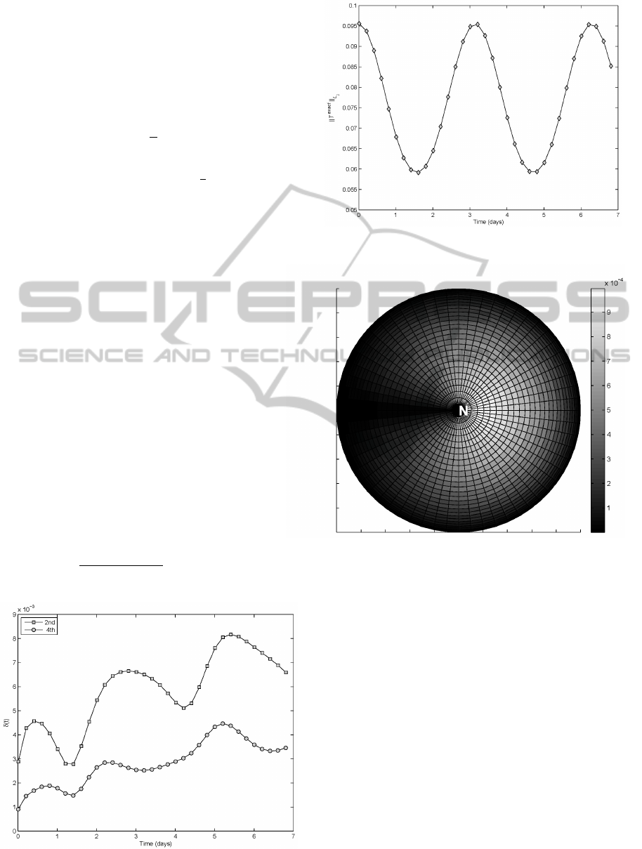
behaviour of the L
2
-norm of the analytical solution.
Problem 2. Let the initial condition be a spot located
at the north pole. We take α = 0 and introduce a non-
constant asymmetric diffusion coefficient of the form
(Fig. 4)
µ(λ,ϕ) = sin
λ
2
sin
2
ϕ. (19)
The asymmetry introduced by sin
λ
2
has the aim to
make sure the grid swap (5)-(6) does not disturb the
solution by introducing any artificial errors near the
poles. If it does, unphysical effects in the solution
will be observed.
The numerical solution computed on the grid 6
◦
×
6
◦
shows that the spot is spreading in accordance with
the diffusion coefficient’s form: the diffusion process
is mainly observed where µ achieves its maximum
(λ = π), whereas less diffusion happens where µ is al-
most negligible (λ ≈ 0) (Figs. 5). No any other effects
are observed (cf. Fig. 4).
Problem 3. To apply the developed schemes to a
nonlinear diffusion problem, we take α = 2 and µ =
1 · 10
−7
, while for the exact solution we choose
T (λ, ϕ,t) = 20 sin ξ cos ϕ cos
2
t + 300,
ξ ≡ ωλ + ϑcos κϕsint. (20)
Then, substituting (20) into (1), for the sources we
find
f (λ,ϕ,t) = −
20µT
α−1
cos
2
t
R
2
cosϕ
( f
1
+ f
2
+ f
3
) + f
4
, (21)
Figure 2: Problem 1: Relative errors δ(t) for the second-
and the fourth-order schemes.
Figure 3: Problem 1: L
2
-norm of the analytical solution
(15).
Figure 4: Problem 2: Form of the diffusion coefficient (19),
pole view.
where
f
1
(λ,ϕ,t) = 20α cos ϕ cos
2
t

ω
2
cos
2
ξ + sin ϕ∗
sinξ(κϑsint cos ξsin κϕcos ϕ + sin ξ sin ϕ)) ,
f
2
(λ,ϕ,t) = T sin ξ

sin
2
ϕ − cos
2
ϕ − ω
2

,
f
3
(λ,ϕ,t) = κϑ sint cos ϕ ∗

20αcosξsinκϕcosϕcos
2
t∗
(κϑsint cos ξsin κϕcos ϕ + sin ξ sin ϕ)−
T (κϑ sint sin ξ sin
2
κϕcosϕ+
cosξ(κcosκϕcosϕ − 3 sin κϕ sin ϕ))] ,
f
4
(λ,ϕ,t) = 20 cos ϕ

ϑcosκϕcosξcos
3
t−
sinξsin2t) . (22)
We assume ω = 7, ϑ = 7π/2, κ = 3.
In Fig. 6 we plot graphs of the relative errors δ(t)
in time for the second- and the fourth-order schemes,
SIMULATION OF NONLINEAR DIFFUSION ON A SPHERE
27

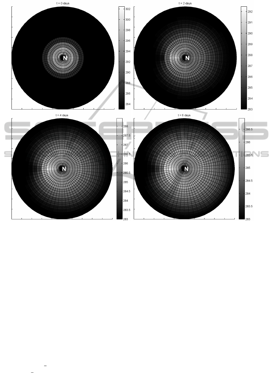
Figure 5: Problem 2: Diffusion of a (north-)pole-located spot at various time moments (4th-order scheme, pole view).
while in Fig. 7 we show the temporal behaviour of the
L
2
-norm of the exact solution (20).
One can observe that the fourth-order scheme
yields better results than the second-order one
(maxδ(t) 0.05 vs. 0.075). Yet, the relative errors
demonstrate periodical behaviour, similar to the an-
alytical solution, which indicates the operator split-
ting provides accurate approximations to the original
unsplit differential problem. As for period doubling,
this phenomenon is due to the structure of the solution
(20).
As for the solution itself (Figs. 8), it is properly
behaving according to the term sinξ. Specifically, as
the time t grows, the sinusoid begins travelling to the
west at low latitudes and to the east at high ones, since
the phase shift ϑcos κϕsint is positive for ϕ ≈ 0 and
negative for ϕ ≈ ±
π
2
at small times. When the time
comes to t =
π
2
, the direction of rotation is changed
to the opposite one, etc. This is exactly what one can
observe in Figs. 8 for a few time moments.
4 CONCLUSIONS
We have developed a new numerical technique for
the simulation of nonlinear diffusion processes in the
spherical geometry when the computational domain
is the entire sphere. The core of the technique con-
sists in performing splitting of the original operator
by coordinates and subsequent grid swap. This ap-
proach allows constructing second- and fourth-order
finite difference schemes efficiently implementable as
systems of linear algebraic equations with band ma-
trices. Numerical tests have proved the approach to
provide highly accurate results and to be suitable for
simulating both linear and nonlinear diffusion phe-
nomena on a sphere.
SIMULTECH 2011 - 1st International Conference on Simulation and Modeling Methodologies, Technologies and
Applications
28

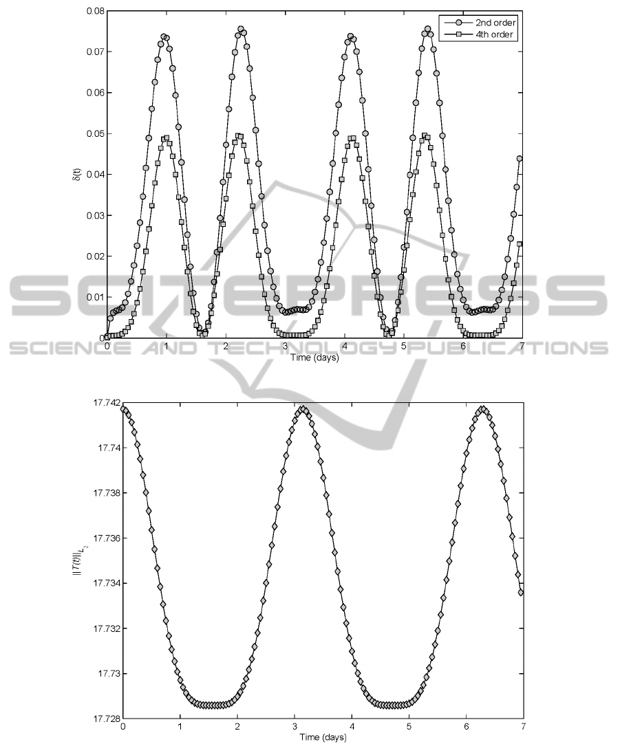
Figure 6: Problem 3: Relative errors δ(t) for the second- and the fourth-order schemes.
Figure 7: Problem 3: L
2
-norm of the analytical solution (20).
ACKNOWLEDGEMENTS
This research was partially supported by the grants
No. 14539 and No. 26073 of the National System
of Researchers of Mexico (SNI), and is part of the
projects PAPIIT-UNAM IN105608, FOSEMARNAT-
CONACyT 2004-01-160, Mexico.
SIMULATION OF NONLINEAR DIFFUSION ON A SPHERE
29

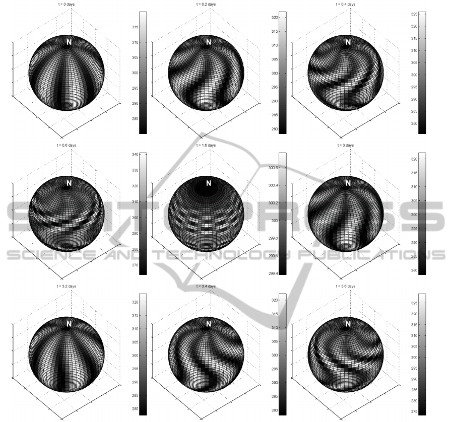
Figure 8: Problem 3: Numerical solution at several time moments (2nd-order scheme, grid 6
◦
× 6
◦
).
REFERENCES
Bear, J. (1988). Dynamics of Fluids in Porous Media. Dover
Publications, New York.
Gibou, F. and Fedkiw, R. (2005). A fourth order accurate
discretization for the laplace and heat equations on ar-
bitrary domains, with applications to the stefan prob-
lem. J. Comput. Phys., 202:577–601.
Lacey, A. A., Ockendon, J. R., and Tayler, A. B. (1982).
“waiting-time” solutions of a nonlinear diffusion
equation. SIAM J. Appl. Math., 42:1252–1264.
Marchuk, G. I. (1982). Methods of Computational Mathe-
matics. Springer-Verlag, Berlin.
Peletier, L. A. (1981). The porous media equation. In Am-
mam, H. and Bazley, N., editors, Applications of Non-
linear Analysis in the Physical Sciences, pages 229–
241. Pitman, Boston.
Press, W. H., Teukolsky, S. A., Vetterling, W. T., and Flan-
nery, B. P. (2007). Numerical Recipes: The Art of Sci-
entific Computing. Cambridge University Press, Cam-
bridge.
Seshadri, R. and Na, T. Y. (1985). Group Invariance in En-
gineering Boundary Value Problems. Springer-Verlag,
New York.
Skiba, Y. N. and Filatov, D. M. (2011). On an efficient
splitting-based method for solving the diffusion equa-
tion on a sphere. Numer. Meth. Part. Diff. Eq., 27:doi:
10.1002/num.20622.
Wu, Z., Zhao, J., Yin, J., and Li, H. (2001). Nonlinear Dif-
fusion Equations. World Scientific Publishing, Singa-
pore.
SIMULTECH 2011 - 1st International Conference on Simulation and Modeling Methodologies, Technologies and
Applications
30