
MONOCULAR VS BINOCULAR 3D REAL-TIME BALL TRACKING
FROM 2D ELLIPSES
Nicola Greggio
⊘,‡
, Jos´e Gaspar
‡
, Alexandre Bernardino
‡
and Jos´e Santos-Victor
‡
⊘
ARTS Lab - Scuola Superiore S. Anna, Polo S. Anna Valdera, Viale R. Piaggio 34, 56025 Pontedera, Italy
‡
Instituto de Sistemas e Rob´otica, Instituto Superior T´ecnico, 1049-001 Lisboa, Portugal
Keywords:
Machine vision, Pattern recognition, Least-square fitting, Algebraic distance.
Abstract:
Real-Time tracking of elliptical objects, e.g. a ball, is a well studied field. However, the question between a
monocular and binocular approach for 3D objects localization is still an open issue. In this work we imple-
mented a real-time algorithm for 3D ball localization and tracking from 2D image ellipse fitting with calibrated
cameras. We will exploit both approaches, together with their own characteristics. Our algorithm features the
following key features: (1) a real-time video segmentation by means of a Gaussian mixture descriptor; (2)
a closed-form ellipse fitting algorithm; and (3) a novel 3D reconstruction algorithm for spheres from the 2D
ellipse parameters. We test the algorithm’s performance in several conditions, by performing experiments in
virtual scenarios with ground truth. Finally, we show the results of monocular and binocular reconstructions
and evaluate the influence of having prior knowledge of the ball’s dimension and the sensitivity of binocular
reconstruction to mechanical calibration errors.
1 INTRODUCTION
3D object localization and tracking are leading sub-
jects robotics and computer vision. The current
ever and ever improvements in hardware capabili-
ties (framegrabbers, motor controllers) require ever
and ever more sophisticated techniques and algo-
rithms to coope with. This is because the correct ob-
ject/target identification in terms of 3D position, di-
mension, velocity, and trajectory is of primary impor-
tance to many applications. Vehicle guidance (Stentz,
2001) (Shi et al., 2007), rescue (Carpin et al., 2006)
(S. Balakirsky et al., 2007), soccer robots (Menegatti
et al., 2008) (Assfalg et al., 2003), or surveillance
systems (Ottlik and Nagel, 2008) (Davis et al., 2006)
are only few examples of fields that exploit this con-
cept. In general unstructured and dynamic environ-
ments, tracking techniques must be robust, to cope
with world uncertainty and sensor noise, and compu-
tationally efficient to provide fast reaction times to un-
expected events.
Robustness is closely linked to the environment
the application has to perform into. For instance, in
industrial applications (i.e. in structured scenarios) a
non-robust algorithm can perform well because of the
absence of disturbances. However, in non-constrained
scenarios this is no longer true: changes in color,
shape and speed of the object can significantly per-
turb object identification and tracking. For instance
in outdoor vision and robotics applications, like video
surveillance and rescue robots, there is the need of a
substantial adaptability toward the changing lighting
and color conditions. The other fundamental issue re-
quired by a vision identification algorithm is its com-
putational efficiency. For example in video surveil-
lance, a precise but very slow algorithm leads to high
(and sometimes unacceptable) latency time between
the image acquisition and its feature extraction. Also
in vision-based control applications, like robotics or
vehicle guidance, low latencies are essential for the
stability and performance properties of the control
loops.
1.1 Related Work
Stereovision tracking requires the usage of two or
more calibrated cameras that capture the same im-
age at the same time from different known positions
and orientation. An addressing example are the two
cameras in a humanoid robot. Each image (left and
right is processed separately in order to isolate the
target). Then, thanks to the known robot’s direct
kinematics and encoders information the target posi-
tion is retrieved by means of geometric triangulation
67
Greggio N., Gaspar J., Bernardino A. and Santos-Victor J..
MONOCULAR VS BINOCULAR 3D REAL-TIME BALL TRACKING FROM 2D ELLIPSES.
DOI: 10.5220/0003543400670073
In Proceedings of the 8th International Conference on Informatics in Control, Automation and Robotics (ICINCO-2011), pages 67-73
ISBN: 978-989-8425-75-1
Copyright
c
2011 SCITEPRESS (Science and Technology Publications, Lda.)

(Forsyth and Ponce, 2002). In 2004, Kwolek devel-
oped a method for tracking human heads with a mo-
bile stereovision camera (Kwolek, 2004). He charac-
terized faces by first performing a color filtering, and
then by modeling the head in the 2D image domain
as an ellipse. Therefore, they formulated the tracking
problem as a probabilisticone in which a particle filter
is used to approximate the probability distribution by
a weighted color cue, shape information, and stereovi-
sion sample collection. In 2011, Greggio et Al. imple-
mented a 3D tracker for the iCub platform featuring
an ellipse pattern recognition algorithm for the target
description (Greggio et al., 2011). In their work, the
authors performed a simple color based image filter-
ing in order to evidence a green ball. Then, the 2D in-
formation obtained with both the iCub’s cameras has
been processed by the ellipse detector, and the results
triangulated in order to reconstruct the ball’s position.
On the other hand, monocular tracking features
the usage of a single camera. Therefore all the tri-
angulation information are lost, making this category
more challenging than the previous one. Many ex-
ertions go toward the human beings tracking. Face
tracking is one of the most important application for
both video surveillance or simple people detection. In
their work, Gokturk et Al. proposed tho apply the
Principal Component Analysis to learn all the possi-
ble facial deformations (Gokturk et al., 2001). Then,
they tracked pose and deformation of the face from an
image sequence. Fossati et Al. used a motion model
to infer 3-D poses between consecutive detections for
identifying key postures for recognizing people seen
from arbitrary viewpoints by a single and potentially
moving camera (Fossati et al., 2007). In 2010 An-
driluka et Al. proposed a people spatial pose estima-
tion technique based on three stages: Initial estimate
of the 2D articulation from single frames, data asso-
ciation across frames, and recovering 3D pose (An-
driluka et al., 2010).
1.2 Main Contributions
In this work we present a real-time algorithm that
robustly segments color blobs modeled by a finite
Gaussian mixture model, following the approach pro-
posed in (Greggio et al., 2010a) and in (Greggio et al.,
2010b). This is an essential pre-processing step that
allows the identification of connected components in
the image where the remaining phases will be ap-
plied. Then, we present a novel algorithm to com-
pute the 3D position of a world sphere correspond-
ing to the projected ellipse in the camera. We per-
formed several experiments in the simulator of the
iCub robot (Tikhanoff et al., 2008) in order to verify
our approach’s performance in a realistic context. We
compare, the reconstructions obtained with monocu-
lar and binocular approaches with ground truth data.
Besides, we consider the existence or absence of a
priory knowledge about the ball’s dimensions.
1.3 Paper Organization
This paper is organized as follows. In sec. 2 we
will describe our mapping from 2D to 3D coordinates.
Then, in sec. 3 we will describe our experimental set-
up and we will discuss our results. Finally, we will
conclude and point out directions for future work in
sec. 4.
2 3D RECONSTRUCTION FROM
ELLIPSES
In this section we describe how to reconstruct the 3D
location of the ball given monocular and binocular
images of the ball silhouette and, in the monocular
case, the knowledge of the ball radius.
2.1 Projection Equation
Describing the ball as a quadric surface, solution of
the quadratic equation:
X
T
QX = 0, (1)
where X = [x y z 1]
T
is a point of the projective space
belonging to the ball surface, and its imaged silhou-
ette (ellipse) as a conic:
m
T
Cm = 0 (2)
where m = [u v 1]
T
is a point of the projective plane
belonging to the imaged silhouette, then the projec-
tion of the ball Q to the ellipse C
1
is simply (Cross
and Zisserman, 1998):
C
∗
∼ PQ
∗
P
T
(3)
where P is a 3× 4 projection matrix,C
∗
= ad j(C) and
Q
∗
= ad j(Q) are the dual conic and the dual quadratic
of C and Q respectively, and ∼ denotes equality up to
a scale factor.
2.2 Monocular Reconstruction
Given the particular case of a spherical ball, the
quadratic Q has a simplified form. Considering a
1
In order to simplify the notation, we refer the parameter ma-
trices Q and C interchangeably with the associated quadratic and
conic equations.
ICINCO 2011 - 8th International Conference on Informatics in Control, Automation and Robotics
68

ball with radius R centered at the origin, one has
Q
0
= diag(1,1,1, −R
2
). Translation of the ball to a
generic 3D location t = [t
x
t
y
t
z
]
T
is obtained by apply-
ing the homogeneous coordinates transformation T to
Q
0
as Q = TQ
0
T
T
, with T = [I
3
− t; 0
T
3
1] where I
3
is a 3× 3 identity matrix and 0
3
is a vector of zeros.
The translated quadratic has therefore the form:
Q =
I
3
−t
−t
T
t
T
t − R
2
(4)
Noting that C and Q are symmetric matrices,
then the adjoint matrices coincide with their inverses.
Hence, the projection equation Eq.3 can be written as
C
−1
∼ PQ
−1
P
T
, with:
Q
−1
=
I
3
− tt
T
/R
2
−t/R
2
−t
T
/R
2
−1/R
2
(5)
Considering, without loss of generality, that a
camera has its coordinate frame coincident with the
world frame P = K[I
3
0
3
], where K denotes the in-
trinsics parameters matrix, one obtains C
−1
∼ K(I
3
−
tt
T
/R
2
)K
T
. Given that K is an invertible matrix one
obtains the normalized projection equation:
I
3
− tt
T
/R
2
∼ K
−1
C
−1
K
−T
(6)
Computing the characteristic equation of the LHS
of Eq.6, det(I
3
− tt
T
/R
2
− λI
3
) = 0 one finds that the
LHS matrix has the eigenvalues λ
1,2,3
= {1,1,1 −
kt/Rk
2
}
2
. The two unitary eigenvalues of the LHS
imply that the RHS has also two equal eigenvalues,
but usually not-unitary given that the equality is only
up to a scale factor. However, this observation allows
finding a scale for the RHS that makes it equal to the
LHS. The scaling has just to impose that the equal
eigenvalues of the RHS are scaled to become unitary,
which can be done by sorting the three eigenvalues
and selecting the middle one.
More specifically, defining H as the normalized
conic of the RHS of Eq.6, i.e. H = K
−1
C
−1
K
−T
, one
removes the scale ambiguity by computing the me-
dian of the eigenvalues:
I
3
− tt
T
/R
2
= H/median(eig(H)) (7)
where eig(H) denotes a function returning the set of
three eigenvalues of H.
Removed the scale ambiguity, Eq.7 allows solving
easily for the direction of the ball location v = t/R.
Denoting H
2
= I
3
− H/median(eig(H)), one obtains
2
Despite appearing that λ
3
= 1 − kt/Rk
2
can be zero, hence
posing questions about the existence of Q, this is not a case of prac-
tical importance since λ
3
= 0 implies ktk = R, meaning that the ball
would touch the camera projection center which is not possible in
practice.
vv
T
= H
2
and the direction of the ball location in the
camera frame is:
v =
s
1
p
H
2(1,1)
s
2
p
H
2(2,2)
s
3
p
H
2(3,3)
(8)
where s
1
,s
2
,s
3
denote the signs of the components
of v. Assuming that the ball is in front of the cam-
era, and the optical axis of the camera is the z axis,
pointing forward, then s
3
= +1 and one can compute
s
1
= sign(H
2
(1,3)),s
2
= sign(H
2
(2,3)) where sign(.)
is the sign function returning +1,−1,0 for positive,
negative or null arguments respectively. Finally, given
the ball radius, R computing the ball location in the
camera frame coordinate, t is just a scaling of the
computed direction:
t = Rv. (9)
Computing the ball location in world coordinates,
w
t, given a generic projection matrix, P = K[
c
R
w
c
t
w
],
proceeds as before, firstly using just the intrinsic pa-
rameters K, and than correcting the computed pose to
the world coordinates frame:
w
t =
c
R
w
t +
c
t
w
(10)
Note that even if P is not given in a factorized form,
the intrinsic K and extrinsic parameters
c
R
w
,
c
t
w
can
be extracted from P using QR factorization as de-
scribed in (Hartley and Zisserman, 2000).
2.3 Binocular Reconstruction
Considering a binocular vision system, Eq.3 is repli-
cated for the two cameras:
C
−1
1
∼ P
1
Q
−1
P
T
1
C
−1
2
∼ P
2
Q
−1
P
T
2
where P
1
and P
2
denote the two projection matrices,
possibly having different intrinsic matrices, K
1
,K
2
,
rotation matrices,
c1
R
w
,
c2
R
w
, and camera centers,
c1
t
w
,
c2
t
w
.
In the case of knowing the radius of the ball, R
then the monocular reconstruction methodology can
be applied twice, resulting in two estimates of the ball
location,
w
t
1
,
w
t
2
, from which one can obtain a final
estimate as the mean of the two estimates,
w
t = (
w
t
1
+
w
t
2
)/2.
In case of not knowing the radius of the ball, a
binocular (stereo) setup still allows obtaining depth
estimates by triangulation, provided that the setup
has a not-null baseline, i.e. different camera cen-
ters,
w
t
c1
6=
w
t
c2
where
w
t
ci
= −
ci
R
−1
w
ci
t
w
and
w
t
ci
=
−P
−1
i(1:3,1:3)
P
i(1:3,4)
for i = 1, 2. Using Eq.8, one ob-
tains two directions to the ball location, v
1
,v
2
, which
MONOCULAR VS BINOCULAR 3D REAL-TIME BALL TRACKING FROM 2D ELLIPSES
69

can be converted to a common (world) coordinate
system,
w
v
i
=
ci
R
−1
w
v
i
, i = 1, 2. The ball location
can therefore be obtained by scaling these directions,
starting at the camera centers,
w
t
ci
, and finding the
closest to an intersection point in a least squares
sense:
(α
∗
,β
∗
) = arg
α,β
minkα
w
v
1
+
w
t
c1
− (β
w
v
2
+
w
t
c2
)k
2
.
(11)
Collecting α, β into a vector, the cost function of
Eq.11 can be rewritten as
A[α β]
T
+ b
2
with A =
[
w
v
1
w
v
2
] and b =
w
t
c1
−
w
t
c2
, thus having a solution
[α
∗
β
∗
]
T
= −(A
T
A)
−1
A
T
b. The ball location can be
estimated just using the scaling factor α, but is more
convenient to use also β:
w
t = (α
∗w
v
1
+
w
t
c1
+ β
∗w
v
2
+
w
t
c2
)/2. (12)
Similarly, the ball radius could be obtained simply as
R = α
∗
, but once more is more convenient to average
the scalings R = (α
∗
+ β
∗
)/2.
3 EXPERIMENTS
3.1 Experimental Set-up
The experimental set-up consists in a virtual world
(the iCub simulator) observed by the robot’s stereo
cameras.The world is constituted by a textured back-
ground, a uniformly colored table and uniformly col-
ored objects, including a ball which will be the subject
of tracking. The ball trajectory is an helix with a di-
ameter of 2m, starting 1.5m away from the robot and
moving with uniform velocity until 2.5m.
50 100 150 200 250 300 350 400 450 500 550
50
100
150
200
250
300
350
400
450
500
550
(a)
−1.5
−1
−0.5
0
0.5
1
1.5
−2
−1
0
−1.5
−1
−0.5
0
0.5
1
1.5
y
x
z
(b)
Figure 1: Left: first image of the sequence used for evalu-
ation. Right: ball’s motion follows an helicoidal trajectory
moving away from the robot.
Fig. 1 shows both the simulator scenario and the
3D helicoidal imposed trajectory. The reason to use a
simulated world in the evaluation of the algorithm is
that it allows us to obtain the ground truth 3D position
of the ball and thus compute the absolute tracking er-
ror achieved by different methods. Also, the intrinsic
and extrinsic camera parameters are known which is
useful to rule our errors thad could arise from cam-
era calibration. We show the performance of our im-
age segmentation method with the proposed Gaussian
Mixture segmentation (Greggio et al., 2010a), (Greg-
gio et al., 2010b), and the ellipse fitting algorithm
(LCSE) (Greggio et al., 2010c). Then we evaluate
our method to reconstruct the 3D position of the ball
from the 2D ellipse parameters comparing monocular
and binocular approaches.
3.2 Image Segmentation by Means of
Gaussian Mixtures
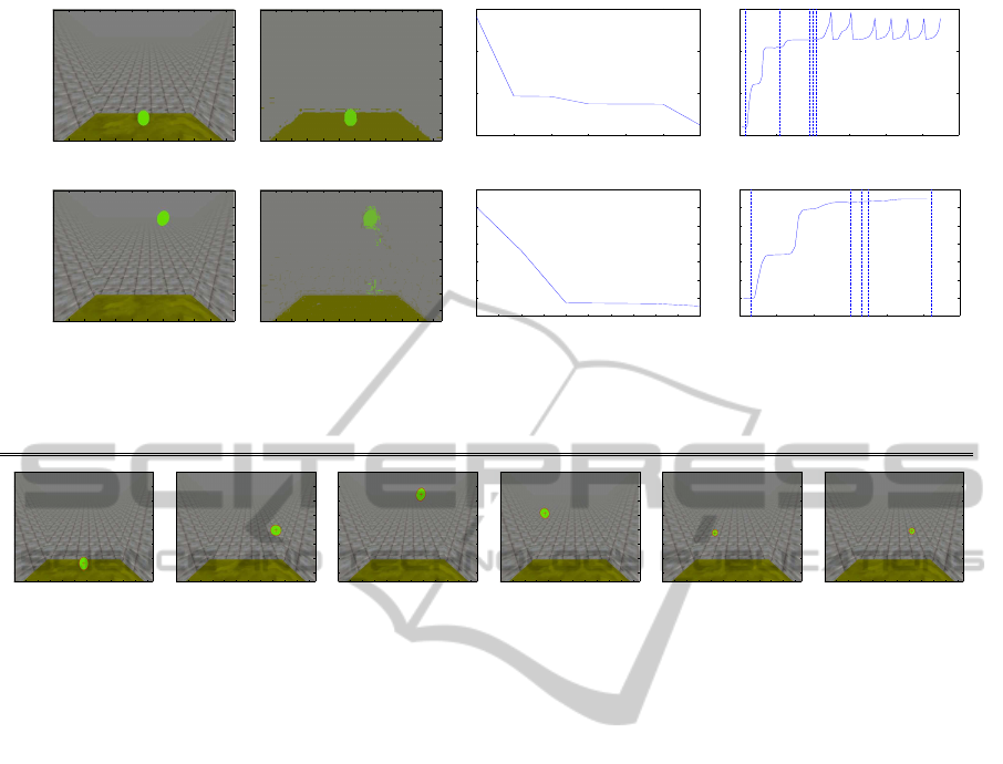
Fig. 2 shows the results of our image segmentation by
means of Gaussian Mixtures algorithm applied to the
images captured from the the iCub simulator. Here,
we collected three sets of images: (1) is a scenario
containing a large ball and a non-spherical object; (2)
contains a small ball over the table; and (3) contains
a small ball against the background. For each set, we
show in Fig. (a) The original image, as captured by
the camera; (b) The color segmented image, (c) the
cost function as function of the number of mixture
components, and (d) the behavior of the whole log-
likelihood as function of the number of iterations.
Learning the right number of color components
(i.e. mixture components) within a colored image
is a difficult task. This is because a general colored
image is supposed to contain a huge number of the
three fundamental color combination, especially on
modern devices. Therefore, the number of mixture
components needed to represent the image at best
rapidly rises up excessively, becoming too high, re-
sulting in an excessive computational burden. Our
approach is able to segment the images with a good
accuracy (all the important features of the image are
reproduced), while performing a lower computational
burden against the other state-of-the-art techniques -
for a deeper comparison see (Greggio et al., 2010b).
3.3 Ellipse Fitting
Fig. 3 shows the results of ellipse fitting algorithm.
Images at top row represent the original images with
the superimposed ellipse.The ellipse fitting technique
performs equally better when the ellipse is bigger or
smaller. Of course, when the pattern’s resolution de-
creases (e.g. when the target is small) the fitting preci-
sion may lack some accuracy, although this is merely
a question of resolution rather than the algorithm it-
self.
ICINCO 2011 - 8th International Conference on Informatics in Control, Automation and Robotics
70
(1)
50 100 150 200 250 300 350 400 450 500 550
50
100
150
200
250
300
350
50 100 150 200 250 300 350 400 450 500 550
50
100
150
200
250
300
350
1 2 3 4 5 6 7
4
4.5
5
5.5
x 10
6
Cost function
Number of components
Cost function
0 20 40 60 80 100 120
−5.5
−5
−4.5
−4
x 10
6
LogLikelihood
Iteration number
LogLikelihood
(a) (b) (c) (d)
(2)
50 100 150 200 250 300 350 400 450 500 550
50
100
150
200
250
300
350
50 100 150 200 250 300 350 400 450 500 550
50
100
150
200
250
300
350
1 1.5 2 2.5 3 3.5 4 4.5 5 5.5 6
4.2
4.4
4.6
4.8
5
5.2
5.4
5.6
x 10
6
Cost function
Number of components
Cost function
0 10 20 30 40 50 60
−5.6
−5.4
−5.2
−5
−4.8
−4.6
−4.4
−4.2
x 10
6
LogLikelihood
Iteration number
LogLikelihood
(a) (b) (c) (d)
Figure 2: Image segmentation by means of Gaussian Mixtures. (a) The original images, as captured by the camera; (b) the
color segmented images, (c) the cost function as function of the number of mixture components, (d) the cost function as
function of the number of iterations, and (e) the behavior of the whole log-likelihood as function of the number of iterations.
50 100 150 200 250 300 350 400 450 500 550
50
100
150
200
250
300
350
50 100 150 200 250 300 350 400 450 500 550
50
100
150
200
250
300
350
50 100 150 200 250 300 350 400 450 500 550
50
100
150
200
250
300
350
50 100 150 200 250 300 350 400 450 500 550
50
100
150
200
250
300
350
50 100 150 200 250 300 350 400 450 500 550
50
100
150
200
250
300
350
50 100 150 200 250 300 350 400 450 500 550
50
100
150
200
250
300
350
(a) (b) (c) (d) (e) (f)
Figure 3: Ball reconstruction image sequence. Images at top row represent the original images with the superimposed ellipse.
3.4 Ball Monocular 3D Localization
In this section we present the results of ball 3D local-
ization using a single camera. Fig. 4 shows the track-
ing errors along time and the 3D reconstructed tra-
jectories. The generated trajectories are shown in red
while the estimated trajectory is represented in blue.
Due to the similarity among the analyzed ellipse fit-
ting methods, in the following experiments we only
use the LCSE ellipse fitting approach (Greggio et al.,
2010c).
We can observe that the reconstructed trajectory
follows closely the true one. The tracking errors grow
slightly for increasing distances, which is a natural
consequence of the decreasing size of the ellipse in
the image and the consequent increase of discretiza-
tion errors and estimation variance. Anyway, the ab-
solute error is always kept below 7cm.
3.5 Comparison between Monocular
and Binocular Reconstructions
In this section we perform the reconstruction of the
ball’s position using a binocular approach. The used
baseline is 10cm, matching approximately the struc-
ture of the iCub robot head. We consider two sce-
narios corresponding to cases where prior knowledge
of the ball radius is absent or present: (i) when ball
radius is unknown we use stereo triangulation, as de-
scribed in section 2.3; (ii) when ball radius is known
we use the mean of the two monocular reconstruc-
tions associated to each of the cameras of the binocu-
lar pair. Furthermore, for the binocular case, we con-
sider the possibility of having uncertainty in the ver-
gence angle formed by the cameras. This is a com-
mon case in robots with moving eyes and is due to
either mechanical effects (backlash, miscalibration)
or asynchronous acquisition of image and motor an-
gles. Results are shown in Fig. 5. The top row shows
the results of stereo triangulation with unknown ball
radius. It is obvious a bigger variance of the esti-
mate with respect to the monocular case, even in the
absence of vergence angle errors (compare Fig. 5(a)
and (d)). This shows the well known sensitivity of
the stereo triangulation algorithm to small errors in
the input data for small baselines. If the ball size is
known, the binocular method copes much better with
vergence angle error (Fig. 5(e) vs (b) and (c)). How-
ever, if the ball size is known, the monocular method
shows roughly the same performance (Fig. 5(d) vs
(e)).
4 CONCLUSIONS
This paper presents a real-time 3D ball tracking sys-
MONOCULAR VS BINOCULAR 3D REAL-TIME BALL TRACKING FROM 2D ELLIPSES
71
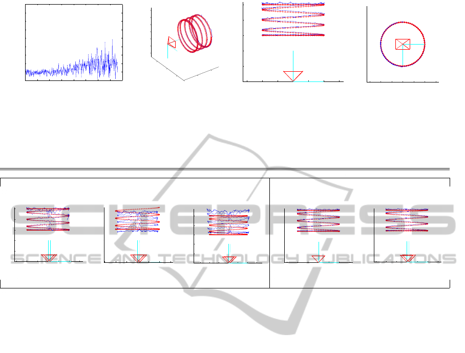
(a) Reconstruction error vs time. (b) 3D reconstructed trajectory
of the ball.
(c) 3D trajectory, top view. (d) 3D trajectory, behind cam-
era frontal view.
Figure 4: 3D monocular reconstruction of the trajectory of the ball based on the LCSE ellipse fitting. Ground truth and
reconstructed trajectories are in red (circles) and blue (dots). The average reconstruction error is 2.8cm for reconstruction
depths larger than 1m.
STEREO TRIANGULATION MONOCULAR RECONSTRUCTION
(a) (b) (c) (d) (e)
Figure 5: Comparing monocular and binocular reconstruction. The left set (a-b-c) shows stereo triangulation, when ball size
is unknown. Stereo reconstruction with zero, −0.2
o
or +0.2
o
vergence errors (a, b and c). The bottom set (d-e) considers
known ball size. Monocular reconstruction (d). Average of two monocular reconstructions, with vergence error of +0.2
o
(e).
tem including all processing stages, from image seg-
mentation, 2D feature extraction and 3D reconstruc-
tion. All stages of the processing pipeline were devel-
oped taking both quality and computation time into
account and are carefully described in the paper. The
segmentation algorithm uses a clustering based ap-
proach in joint color-space coordinates, using a novel
greedy optimization of Gaussian Mixture parameters
that overcomes related techniques in video segmen-
tation. The 2D ellipse fitting method was designed
for improved robustness to singular cases and is com-
petitive with alternative methods. The 3D reconstruc-
tion method is simple, elegant and makes effective of
all ellipse parameters obtained from the image. We
performed experiments with a realistic simulator of
the iCub robot. The full tracking method was evalu-
ated by comparing tracking errors with ground truth
values. Monocular and binocular approaches were
tested, including the presence of errors in vergence
angle measurements. This is a frequentcase in robotic
heads with moving vergence and the results obtained
confirmed our empirical tests on the iCub robot: Ver-
gence angle errors propagate significantly to 3D re-
construction errors in this robot. We showed that a
priori knowledge of the ball radius can reduce signif-
icantly the variance of the 3D estimates. Although it
may not be possible in practice to obtain this knowl-
edge in advance, our future work will focus on the
online estimation of the ball size and the demonstra-
tion of its influence in the 3D reconstruction quality.
ACKNOWLEDGEMENTS
We thank Cecilia Laschi and Paolo Dario for their
support. This work was supported by the Euro-
pean Commission, Project IST-004370 RobotCub and
FP7-231640 Handle, and by the Portuguese Gov-
ernment - Fundac¸˜ao para a Ciˆencia e Tecnologia
(ISR/IST pluriannual funding) through the PIDDAC
program funds and through the projects BIO-LOOK,
PTDC / EEA-ACR / 71032 / 2006, and DCCAL,
PTDC / EEA-CRO / 105413 / 2008.
REFERENCES
Andriluka, M., Roth, S., and Schiele, B. (2010). Monocular
3d pose estimation and tracking by detection. IEEE
Conference on Computer Vision and Pattern Recogni-
tion (CVPR 2010), San Francisco, USA.
ICINCO 2011 - 8th International Conference on Informatics in Control, Automation and Robotics
72

Assfalg, J., Bertini, M., Colombo, C., Del Bimbo, A., and
Nunziati, W. (2003). Semantic annotation of soccer
videos: automatic highlights identifcation. Computer
Vision and Image Understanding, 92:285–305.
Carpin, S., Lewis, M., Wang, J., Balakirsky, S., and Scrap-
per, C. (2006). Bridging the gap between simulation
and reality in urban search and rescue”. In Robocup
2006: Robot Soccer World Cup X.
Cross, G. and Zisserman, A. (1998). Quadric reconstruction
from dual-space geometry. Int. Conf. on Comp. Vision
(ICCV), pages 25–31.
Davis, J. W., Morison, A. W., and Woods, D. D. (2006). An
adaptive focus-of-attention model for video surveil-
lance and monitoring. Machine Vision and Applica-
tions, 18(1):41–64.
Fitzgibbon, A., Pilu, M., and Fisher, R. (1999). Direct least
square fitting of ellipses. IEEE Trans. PAMI, 21:476–
480.
Forsyth, D. A. and Ponce, J. (2002). Computer Vision: A
modern approach. Prentice Hall, NY.
Fossati, A., Dimitrijevic, M., Lepetit, V., and Fua, P. (June
17-22, 2007). Bridging the gap between detection and
tracking for 3d monocular video-based motion cap-
ture. IEEE Conference on Computer Vision and Pat-
tern Recognition, Minneapolis, pages 1–8.
Gokturk, S., Bouguet, J., and Grzeszczuk, R. (2001).
A data-driven model for monocular face tracking.
ICCV01, pages 701–708.
Greggio, N., Bernardino, A., Laschi, C., Dario, P., and
Santos-Victor, J. (2010a). Self-adaptive gaussian mix-
ture models for real-time video segmentation and
background subtraction. IEEE 10th International
Conference on Intelligent Systems Design and Appli-
cations (ISDA), Cairo, Egypt.
Greggio, N., Bernardino, A., Laschi, C., Santos-Victor, J.,
and Dario, P. (2010b). An algorithm for the least
square-fitting of ellipses. IEEE 22th International
Conference on Tools with Artificial Intelligence (IC-
TAI 2010), Arras, France.
Greggio, N., Bernardino, A., Laschi, C., Santos-Victor, J.,
and Dario, P. (2011). Real-time 3d stereo tracking and
localizing of spherical objects with the icub robotic
platform. Journal of Intelligent & Robotic Systems,
pages 1–30. 10.1007/s10846-010-9527-3.
Greggio, N., Bernardino, A., and Santos-Victor, J. (2010c).
Sequentially greedy unsupervised learning of gaus-
sian mixture models by means of a binary tree struc-
ture. 11-th International Conference on Intelligent Au-
tonomous Systems (IAS-11) 2010 - Aug 30, Sept 1.
Hartley, R. and Zisserman, A. (2000). Multiple view geom-
etry in computer vision. Cambridge University Press.
Kwolek, B. (2004). Real-time head tracker using color,
stereovision and ellipse fitting in a particle filter. IN-
FORMATICA, 15(2):219–230.
Maini, E. S. (2006). Enhanced direct least square fitting of
ellipses. IJPRAI, 20(6):939–954.
Menegatti, E., Silvestri, G., Pagello, E., Greggio, N., Maz-
zanti, F., Cisternino, A., Sorbello, R., and Chella, A.
(2008). 3d realistic simulations of humanoid soccer
robots. International Journal of Humanoid Robotics,
5(3):523–546.
Ottlik, A. and Nagel, H.-H. (2008). Initialization of model-
based vehicle tracking in video sequences of inner-
city intersections. International Journal of Computer
Vision, 80(2):211–225.
S. Balakirsky, S. C., A.Kleiner, Lewis, M., Visser, A.,
Wang, J., and Ziparo, V. (2007). Towards heteroge-
neous robot teams for disaster mitigation: Results and
performance metrics from robocup rescue. Journal of
Field Robotics.
Shi, Y., Qian, W., Yan, W., and Li, J. (2007). Adaptive depth
control for autonomous underwater vehicles based on
feedforward neural networks. International Journal of
Computer Science & Applications, 4(3):107–118.
Stentz, A. (2001). Robotic technologies for outdoor in-
dustrial vehicles. Unmanned ground vehicle tech-
nology. Conference No. 3, Orlando FL, ETATS-UNIS
(16/04/2001), 4364:192–199.
Tikhanoff, V., Fitzpatrick, P., Nori, F., Natale, L., Metta,
G., and Cangelosi, A. (2008). The icub humanoid
robot simulator. International Conference on Intel-
ligent RObots and Systems IROS, Nice, France.
MONOCULAR VS BINOCULAR 3D REAL-TIME BALL TRACKING FROM 2D ELLIPSES
73
