
FAULT DETECTION BASED ON GAUSSIAN PROCESS MODELS
An Application to the Rolling Mill
Dani Juricic
1
, Pavel Ettler
2
and Jus Kocijan
1
1
Department of Systems and Control, Jozef Stefan Institute, Jamova 39, Ljubljana, Slovenia
2
COMPUREG Plzen, s.r.o., 306 34 Plzen, Czech Republic
Keywords:
Gaussian process model, Fault detection, Statistical hypothesis test, Cold rolling mill.
Abstract:
In this paper a fault detection approach based on Gaussian process model is proposed. The problem we raise
is how to deal with insufficiently validated models during surveillance of nonlinear plants given the fact that
tentative model-plant miss-match in such a case can cause false alarms. To avoid the risk, a novel model
validity index is suggested in order to quantify the level of confidence associated to the detection results. This
index is based on estimated ‘distance’ between the current process data from data employed in the learning
set. The effectiveness of the test is demonstrated on data records obtained from operating cold rolling mill.
1 INTRODUCTION
It has been widely recognized that design of purpose-
ful process model usually represents the bottleneck
in the diagnostic system design (Venkatasubramanian
et al., 2003).In this paper we investigate a relatively
recent approach named Gaussian process model (GP),
which is a non-parametric description of the nonlinear
process (Rasmussen and Williams, 2006). We address
two issues related to the application of GP in fault de-
tection. First is the residual generation and evaluation,
which is performed by calculating the error between
the true output and that predicted by GP model. The
zero/non-zero qualitative value of the residual is de-
termined by means of the statistical hypothesis test-
ing. Second, we address the problem of on-line as-
sessment of model validity. The aim is to avoid pos-
sible false alarms that might occur due to incorrect
association of the prediction error with process fault
instead of insufficiently accurate process model. A
model validity index is suggested, which quantifies
the level of confidence associated with the detection
results.
The paper is organized as follows. In section 2 the
essentials of GP models are reviewed. In section 3 the
detection procedure is derived. Section 4 focuses on
derivation of the validity index. The ideas are imple-
mented as part of the case study related to the mon-
itoring of cold rolling mills. Finally, conclusions are
drawn and perspectives for future work are given.
2 SYSTEMS MODELLING WITH
GAUSSIAN PROCESSES
A detailed presentation of Gaussian process mod-
els can be found, e.g., in (Rasmussen and Williams,
2006) and some applications in, e.g., (Kocijan and
Likar, 2008).
GP emerges as the result of central limit theo-
rem (CLT). The nonlinear relationship between mea-
sured output y(x(k)) ∈ R and the regressor x(k) ∈ R
D
,
where k is the sample number, can be expressed as a
weighted sum of the eigen-functions Φ
i
(x(k))
y(k) = y(x(k)) =
m
∑
i=1
w
i
Φ
i
(x(k))) + n(k)
where n(k) is zero mean white i.i.d. noise. If w
i
are
zero mean i.i.d and m → ∞ under certain conditions
the CLT returns (Der and Lee, 2005)
y(x(1)),...,y(x(N)) ∼ N (0,Σ
Σ
Σ) (1)
Σ
Σ
Σ =k σ
i, j
k
σ
ij
= cov(y(i)y( j)) = C(x(i),x( j)) = (2)
= ve
−
1
2
(x(i)−x( j))
′
W(x(i)−x( j))
+ v
0
δ
ij
where W = diag(w
1
,w
2
,...,w
D
) are the ‘hyperpa-
rameters’ of the covariance functions C : R
D×2
→ R
(Rasmussen and Williams, 2006), v
0
is the estimated
noise variance, v is the estimate of the vertical scale
of variation, D is the input dimension and δ
ij
is Kro-
necker operator.
437
Juricic D., Ettler P. and Kocijan J..
FAULT DETECTION BASED ON GAUSSIAN PROCESS MODELS - An Application to the Rolling Mill.
DOI: 10.5220/0003541304370440
In Proceedings of the 8th International Conference on Informatics in Control, Automation and Robotics (ICINCO-2011), pages 437-440
ISBN: 978-989-8425-74-4
Copyright
c
2011 SCITEPRESS (Science and Technology Publications, Lda.)

Consider a set of N input vec-
tors X = [x(1),x(2),...,x(N)] of dimen-
sion D and a vector of output data
y = [y(1),y(2),...,y(N)]
T
. Based on the data
set L = X, and given a new input vector x
∗
, we
wish to find the predictive distribution of the cor-
responding output y
∗
. For a new test input x
∗
, the
predictive distribution of the corresponding output is
p(y
∗
|x
∗
,(X,y)) ∼N (m(y
∗
),σ
2
(y
∗
)), i.e. is Gaussian,
with mean and variance
m(y
∗
) = k(x
∗
)
T
Σ
Σ
Σ
−1
y (3)
σ
2
(y
∗
) = k(x
∗
) − k(x
∗
)
T
Σ
Σ
Σ
−1
k(x
∗
) (4)
where k(x
∗
) = [C(x
1
,x
∗
),...,C(x
N
,x
∗
)]
T
is the N ×
1 vector of covariances between the test and training
cases and k(x
∗
) = C(x
∗
,x
∗
) is the covariance between
the test input and itself.
The estimation of the hyper-parameters of the co-
variance function is done by maximizing the log-
likelihood of the parameters. This can be computa-
tionally demanding since the inverse of the (N ×N)
data covariance matrix has to be calculated at every it-
eration. The cross-validation fit of predictions is usu-
ally evaluated by log predictive density error (Kocijan
and Likar, 2008),
LD =
1
2
log(2π) +
1
2N
N
∑
i=1
(log(σ
2
i
) +
e
2
i
σ
2
i
), (5)
where y
i
, e
i
= ˆy
i
−y
i
and σ
2
i
are the system’s output,
the prediction error and the prediction variance of the
i-th element of output.
3 DETECTION PROCEDURE
BASED ON GP MODELS
As measured output y(k) and the predicted ˆy(k) are
both stochastic processes, detection will employ
the realization of pairs { y(1),x(1)},....,{y(i),x(i)}
and {ˆy(1),x(1)}, ...., {ˆy(i),x(i)} computed with GP
model. The difference between the actual y(k) and
the predicted ˆy(k) is referred to as residual.
3.1 Residual Generation with GPs
The prediction error can be set as follows:
ε(k) = y(k) −m(x(k)) (6)
Intuitively, if the prediction error is low, there
might be a good reason to infer that no fault affects
the system. High prediction error, on the other hand,
might mean either
• a fault is present in the system (e.g. instrument
reading) or
• the process operation reached a region for which
the process model is not appropriate, i.e. the vec-
tor x is far from the learning set L .
Assume we have a vector of residualsε
ε
ε(k) and the
associated covariance matrix S(k) as follows
ε
ε
ε(k) = [ε(k −M + 1),ε(k−M+ 2),...,ε(k)]
T
(7)
S(k) = E{ε
ε
εε
ε
ε
T
} = C(X
X
X(k),X
X
X(k))
− C(X
X
X(k),X
X
X
L
)Σ
Σ
Σ
−1
C(X(k),X
L
)
T
where X(k) = [x(k −M + 1),x(k−M + 2),...,x(k)],
X
L
⊂ L and the matrix
C(X
X
X(k),X
X
X(k)) =kC(x
x
x
i
,x
x
x
j
),x
x
x
i
∈X
X
X(k),x
x
x
j
∈X
X
X
L
) k .
The problem we have now is to decide whether a bias
f
y
in predicted output y(t) is present (f
y
6= 0) or not
(f
y
= 0).
3.2 Detection Rule based on a Statistical
Test
If there is no fault in the system the distribution of
ε
ε
ε(k) should read
ε
ε
ε(k) ∼N (0,S(k)) (8)
A bias error f
y
in the predicted output result in offset
in computedresidual ε(i). We have to choose between
the null hypothesis
H
0
: f
y
= 0
and the alternative
H
1
: f
y
6= 0
One rejects H
0
if the likelihood ratio is such that (Ro-
htagi, 1976)
κ =
p
f
y
=0
(ε
ε
ε(k))
sup
f
y
6=0
p
f
y
6=0
(ε
ε
ε(k))
< τ (9)
Supremum in the denominator is achieved for
µ =
1
T
N
S(k)
−1
ε
ε
ε(k)
1
T
N
S(k)
−1
1
N
(10)
where 1
T
N
= [1,...,1
| {z }
N−times
]
T
From the logarithm of the likelihood ratio test (9)
(with (10) in mind), the followingcondition for reject-
ing the null hypothesis H
0
at the level of significance
β follows
S
N
(k) =
| 1
T
N
S(k)
−1
ε
ε
ε(k) |
q
1
T
N
S(k)
−1
1
N
> c
1−β/2
(11)
Here c
1−β/2
is the significance level taken from the
normal distribution at the degree of significance β.
ICINCO 2011 - 8th International Conference on Informatics in Control, Automation and Robotics
438

4 MONITORING THE
DETECTOR WITH A MODEL
VALIDITY INDEX
The validity of the test (11) can be violated if GP
model is forced to make predictions at the points x
far from the learning set L . In practice, it might of-
ten happen that process model, originally trained in
certain operating region(s), is employed in a new op-
erating region not included in the learning set.
In this paper we rely on the observation that sensi-
tivity is inherent to the Gaussian process models. We
focus on y i.e. the scaled noise-free mapping of input
regressor x, which is related to y as follows
y(x(t)) =
√
v·y(x(t)) + n(t)
y(t) ∼ N (0,
˜
C(x(t),x(t)))
where
˜
C : R
D×2
→ R is modified covariance function
defined by
˜
C(x(i),x( j)) = exp
−
1
2
(x(i) −x( j))
T
W(x(i) −x( j))
Furthermore, note also that x(i) = x( j) implies
y(x(i)) = y(x( j)). Assume L = {x
i
,i = 1,...,N}. Let
the modified covariance matrix of the learning set
L be
˜
Σ
Σ
Σ(L ,L ) = k
˜
σ
ij
=
˜
C(x
i
,x
j
)k,i, j ∈ {1, ...,N}
Now, we start by adopting the notion of the distance
between a new regressor x and the learning set L .
Intuitively, if x = x
k
,k ∈ {1,...,N} then the distance
should be zero.
Proposition 1. Assume the learning set L =
{x
i
,i = 1,...,N} and x is a regressor. The distance
between x
x
x and L is
δ(x,L ) =
˜
C(x, x) −
˜
Σ
Σ
Σ(x,L )
′
˜
Σ
Σ
Σ(L ,L )
−1
˜
Σ
Σ
Σ(x,L ). (12)
In eq. (12) the meaning of
˜
Σ
Σ
Σ(x,L ) is
˜
Σ
Σ
Σ(x,L ) = [
˜
C(x, x(1))...
˜
C(x,x(N))]
′
In the same manner as in case of a single regressor
x one can associate distance to the covariance matrix
of the predicted y(X) conditioned on L . Actually, the
result (12) is extended as follows
D(X,L ) =
˜
Σ
Σ
Σ(X,X) −
˜
Σ
Σ
Σ(X,L )
′
˜
Σ
Σ
Σ(L ,L )
−1
˜
Σ
Σ
Σ(X,L ).
(13)
Again, if X ⊂ L then by borrowing the derivation
from the Proposition 1 one can see that D
D
D = 0
0
0. If X
X
X is
‘far’ from L , D
D
D →I.
Definition 1. The validity index I of the GP model
is proposed as being equivalent to the distance of a set
of regressors from the learning set as follows
I = trace(D(X,L )). (14)
5 EXPERIMENTAL RESULTS
To demonstrate the performance of the above FD
scheme, a case of a cold rolling mill is addressed.
In this process the output strip thickness belongs to
the key process variables. Its control is not trivial and
several approaches are being used to overcome the re-
lated technical problems (Ettler et al., 2007). One of
them relies on exploiting additional redundancybased
on available measured signals and mathematical mod-
els. Therefore, the on-line detection of faults in in-
strumentation and appropriate accommodation is key
for efficient controller design. The estimated value is
directly usable for the thickness control and for mill
operators. The estimator output is in the form of the
probability distribution thus providing clear informa-
tion about reliability of the estimation (Ettler et al.,
2007).
In order to illustrate the method proposed above,
we will focus just on the relationship between thick-
ness H
2
(k), z(k) and rolling force F(k), where k de-
notes the sampling instance. It reads as follows
H
2
(k) = f(z(k),F(k)) (15)
where f is an unknown function which can be de-
scribed by Gaussian process model.
The set of 450 representative input data samples
is used for training of the model (15).The model is
validated with 110 input data samples different from
those used for training.
The proposed statistical test (14) and the validity
index (18) have been used to detect bias in the H
2
sensor. To illustrate the performance a simulation run
consisting of four parts is presented.
First, in the period 0-430 samples the process op-
erates in a fault-free mode. Moreover, in that period
the operating region belongs to the region encom-
passed in the learning set. The response of the detec-
tor is seen in the figure. The window length is taken
M = 50 samples. The process output is well predicted
by the model so that the detector is indicating no-fault
with low value of the validity index.
In the period 430-950 samples an offset f
y
= 100
in H
2
sensor appears. One can see that the test statistic
almost immediately crosses the threshold value thus
indicating the presence of fault. The validity index
stays around zero, indicating that the process is oper-
ating in validated region.
In the third period 950-1450 the process operates
without fault.
At k = 1450 the operating point changes. The
detector receives data not envisaged in the learning
stage, Both the test statistics and validity index grows
indicating that something unusual is going on in the
FAULT DETECTION BASED ON GAUSSIAN PROCESS MODELS - An Application to the Rolling Mill
439
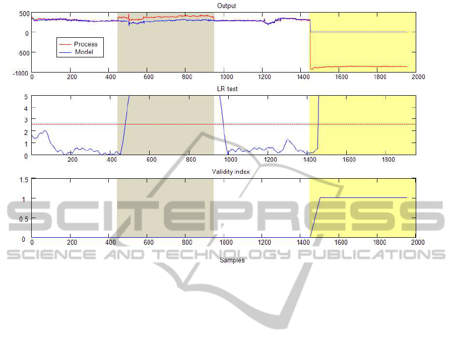
Figure 1: Results obtained over operating records.
process. Without additional information at that stage
it is not possible to distinguish whether the cause is in
fault or in novel operating region.
6 CONCLUSIONS
In this paper we presented a fault detection algorithm
based on Gaussian process model that is suited for
handling instrument faults in nonlinear systems. The
main contributionof the paper regards a validity index
which tells how much should the process model be
trusted when deciding about faults based on data from
current operating region. The idea is implemented in
a Gaussian process model framework, which is suited
for data-driven modelling and requires minimal a pri-
ori knowledge.Further extensions to a wider set of
faults should provide more insight into the potential
of the ideas presented here as well as advantages and
disadvantages compared to other methods.
ACKNOWLEDGEMENTS
The work was supported by the EUROSTARS project
ProBaSensor and by the grants L2-2338 of the Slove-
nian Research Agency and 7D09008 of the Czech
Ministry of Education, Youth and Sports.
REFERENCES
Der R. and D. Lee , 2005. Beyond Gaussian processes: on
the dist, In: Advances in Neural Information Process-
ing Systems. Vol. 18, MIT Press, 275–282.
Ettler P., M. Karny and P. Nedoma , 2007. Model mixing
for long-term extrapolation. Proc. Eurosim Congress,
Ljubljana, Slovenia.
Kocijan J. and Likar, B. , 2008. Gasliquid separator mod-
elling and simulation with Gaussian-process models,
Simulation Modelling Practice and Theory, 16 (8),
910–922.
Rohatgi, V. K., 1976. An Introduction to Probability Theory
and Mathematical Statistics, John Wiley and Sons,
New York, NY.
Venkatasubramanian, V., Rengaswamy, R., Yin, K. and
Kavuri, S. N. , 2003. A review of process fault detec-
tion and diagnosis: Part I: Quantitative model-based
methods, Computers & Chemical Engineering, 27(3),
293–311.
Rasmussen, C. E. Williams,C. K. I. , 2006. Gaussian Pro-
cesses for Machine Learning, MIT Press, Cambridge,
MA.
ICINCO 2011 - 8th International Conference on Informatics in Control, Automation and Robotics
440
