
WHEELED MOBILE MANIPULATOR MODELING FOR TASK
S
PACE CONTROL
Gast´on H. Salazar-Silva
UPIITA, Instituto Polit´ecnico Nacional, Av. IPN 2580, Mexico City, D.F., Mexico
J
aime
´
Alvarez Gallegos
Secretar´ıa de Investigaci´on y Posgrado, Instituto Polit´ecnico Nacional, Mexico City, D.F., Mexico
Marco A. Moreno-Armend´ariz
Centro de Investigaci´on en Computaci´on, Instituto Polit´ecnico Nacional, Mexico City, D.F., Mexico
Keywords:
Robot control, Mobile robots, Robots kinematics.
Abstract:
Mobile manipulators have attracted a lot attention lately because they have many advantages over stationary
manipulator, such as larger a work space than a stationary manipulator could have in practice. However, the
proposed methods in the state of the art to obtain the kinematic model of a mobile manipulator are based in
modeling separately the mobile base and the manipulator arm, and later combining both models.
This paper shows a systematic approach to obtain the kinematic model of mobile manipulators that transforms
in the modeling problem of a stationary manipulator with non-holonomic kinematic constraints in the joints;
it is also showed an example of the application of the method, where the kinematic and dynamic models are
obtained with extensions of the same tools used in stationary robots.
1 INTRODUCTION
A mobile manipulator is a manipulator mounted on
a mobile robot; an example is a manipulator arm
mounted on a mobile robot with differential traction.
Mobile manipulators have many advantages over sta-
tionary manipulator, such as a larger work space. Mo-
bile manipulators can perform the tasks of locomotion
and handling; those tasks have been handled as two
separate problems, for example in (Wang et al., 2008)
the focus is on movement of the mobile base and in
(Joshi and Desrochers, 1986) the task is the motion of
the manipulator arm. However, recently there are lot
of attention to the performance of both tasks simulta-
neously, for example in (Mazur, 2010).
The problem of kinematic modeling of a mobile
manipulator has been attacked by obtaining sepa-
rately the kinematic models of the base and arm ma-
nipulator, and then combining both models (De Luca
et al., 2006). Due to the usefulness of mobile manip-
ulators, it is important to have methods and tools that
allow an easier analysis of the mobile manipulator.
This paper shows an integrated approach to the
kinematic modeling of wheeled mobile manipulators
that apply the same tools used in modeling stationary
robots. This method assumes that the mobile manipu-
lator is a stationary robot which have joints with non-
holonomic constraints; this approach allows the use
of existing tools to obtain the kinematic and dynamic
models, for example the Denavit–Hartenberg param-
eters and geometric Jacobians.
A kinematic modeling scheme for mobile manipu-
lators is presented in (Bayle et al., 2003; Mazur,2010)
where the kinematic models for the mobile platform
and the arm are determined separately. In (De Luca
et al., 2006) a method is presented for combining the
kinematic model of the mobile base with the station-
ary manipulator, but the mobile base and the manipu-
lator are still modeled with different methods. Partic-
ularly interesting example is in (Mazur, 2010), where
both the mobile base and the manipulator have non-
holonomic constraints and yet are modeled by differ-
ent methods.
The outline of this paper is as follows: the kine-
matic modeling of mobile robots is reviewed in Sec-
tion 2. The modeling method proposed in this report,
modeling the mobile manipulator simply as station-
ary manipulators with joints that have kinematic con-
313
H. Salazar-Silva G., Álvarez Gallegos J. and A. Moreno-Armendáriz M..
WHEELED MOBILE MANIPULATOR MODELING FOR TASK SPACE CONTROL.
DOI: 10.5220/0003540203130316
In Proceedings of the 8th International Conference on Informatics in Control, Automation and Robotics (ICINCO-2011), pages 313-316
ISBN: 978-989-8425-75-1
Copyright
c
2011 SCITEPRESS (Science and Technology Publications, Lda.)

straints, is presented in Section 3. In Section 4 a con-
trol for task space is proposed. As an example of the
method, in Section 5 the kinematic and dynamic mod-
els of a 5-degree of freedom (DOF) mobile manipula-
tor are obtained and the implementation of the control
presented in Section 4 is done.
2 KINEMATIC MODEL OF
MOBILE ROBOT
A kinematic model describes the relationship between
the motion of a mechanical system and the actuation
velocities. The motion of a wheeled mobile robot
is characterized by the constraints imposed by the
wheels (Campion et al., 1996); in this section it is
briefly reviewed the issues on kinematic constraints
and the development of kinematics models.
A set of k kinematic constraints restricts the mo-
tion of a mechanical system and can be expressed as
a
i
(q, ˙q) = 0,
where q ∈ R
n
is the configuration variables vector, ˙q∈
R
n
is the configuration velocities vector and n is the
size of the configuration vector, usually called degree
of freedom (DOF), a
i
are scalar functions on q and
˙q. If the function a
i
does not depend on ˙q then the
system is called holonomic, otherwise it is said that
the system is nonholonomic.
There are two kinds of kinematic models as pro-
posed in (Campion et al., 1996). The first is the pos-
ture kinematic model and is a relationship between
the motion on the task space and the motion of the ac-
tuators; for a wheeled mobile robot with differential
traction it can be expressed as (Campion et al., 1996)
˙r
b
(t) = B
b
(q)η
b
(1)
where ˙r
b
(t) ∈ R
p
are the posture velocities on a task
space of dimension p, η
b
(t) ∈ R
n−k
is the vector
which contains the velocities of the actuators, and
B
b
(q) ∈ R
n×(n−k)
is a matrix with its columns are
a base of the null space of the nonholonomic con-
straints.
On the other hand, the configuration kinematic
model is the relationship between the velocities of the
joints variables and the velocities of the actuators and
it is defined as
˙q
b
(t) = S
b
(q)η
b
(2)
where S
b
(q) ∈ R
n×(n−k)
is a matrix with its columns
are also a base of null space of the constraints. It is
also important to note that S(q) is an annihilator of the
kinematic constraints, such that
A(q)
T
S
b
(q) = 0; (3)
this fact can be used to simplify the dynamic model
(De Luca and Oriolo, 1995).
3 MOBILE MANIPULATOR
MODELING
The kinematics of a mobile manipulator is given by
the function f, defined as
r = f(q) (4)
where r is the combined posture of the mobile manip-
ulator and q are the combined generalized coordinates
of the mobile base and the manipulator arm; Thus the
kinematic modeling of a mobile manipulator depends
on finding the Jacobian J,
J =
∂
∂q
f(q) (5)
and which depends in turn on combining the kinemat-
ics of the manipulator and the base mobile.
A method to find the direct kinematics of the
manipulator arm and mobile base, and also allows
combine them, are the homogeneous transformations;
specifically for the mobile manipulator it is defined as
(Li and Liu, 2004):
T
0
n
= T
0
b
T
b
n
where T
0
b
is the homogeneous transformation which
goes from a frame {b} fixed on the mobile base to
a frame {0} fixed on surface on which the mobile
base moves, and T
b
n
is the homogeneous transforma-
tion which goes from a frame {n} fixed on the last
link of the mobile manipulator to the frame {b}; there
is not a standardized method to find the transforma-
tion T
0
b
. It is important to remark that T
0
b
does not
take account of the nonholonomic constraints.
The proposed method is to obtain the forward
kinematics of the mobile base T
0
b
by assuming that the
mobile base is stationary manipulator of b DOF and
considering it a unique kinematic chain, and the ap-
plying a modeling method for stationary robots, such
as the Denavit–Hartenbergmethod. Also it is possible
to obtain the Jacobian J of the whole mobile manipu-
lator from the same geometric method used in station-
ary robots and then is possible to obtain the posture
kinematic model of mobile manipulator
˙r = B(q)η (6)
where η is the vector of the actuation variables and is
defined as
η =
η
T
b
˙q
T
m
T
,
ICINCO 2011 - 8th International Conference on Informatics in Control, Automation and Robotics
314

B(q) is the posture kinematic relation of the mobile
manipulator, defined as
B(q) = J(q)S(q)
S(q) is the configuration kinematic relation for the
whole mobile manipulator
S(q) =
S
b
(q) I
where I is a identity matrix, showing that the config-
uration velocities are identical to the actuation veloci-
ties. Some advantages of the proposed method is that
uses the same methods and computational tools as the
stationary manipulators to obtain the kinematic mod-
els.
4 CONTROL IN TASK SPACE
The control proposed in this paper follows the classi-
cal combination of two control loops in cascade; the
internal loop control uses an inverse dynamics con-
trol. The external control loop is a resolution of ac-
celeration control over the task space. The dynamic
model of a mechanical system with non-holonomic
constraints is defined by a set of n second-order dif-
ferential equations
D(q) ¨q+C(q, ˙q) ˙q+ g(q) = A(q)λ+ S(q)τ
A(q)
T
˙q = 0
(7)
where D(q) ∈ R
n×n
is the inertia matrix for the
system, C(q, ˙q) ∈ R
n×n
is the Coriolis and cross-
velocities matrix, g(q) ∈ R
n
is a vector which repre-
sents the impact of gravity on the links, A(q) ∈ R
n×k
is a matrix in which k kinematics constrains are ex-
pressed, S(q) ∈ R
m×n
in the input matrix, and τ ∈ R
m
are the generalized forces that go into system.
Taking advantage of (3), it is possible to eliminate
the explicit statement of the kinematic constraint in
(7) by applying (1), thus the following reduced order
system is obtained (De Luca and Oriolo, 1995)
˙q = S(q)η
˙
η = −M(q)
−1
m(q,η) + S(q)
T
S(q)τ
(8)
where
M(q) = S(q)
T
D(q)S(q)
m(q,η) = S(q)
T
D(q)
˙
Sη+C(q,Sη)Sη + g(q)
.
A control τ is proposed such that it cancels the dy-
namics in (8)
τ = (S(q)
T
S(q))
−1
m(q,η) + (S(q)
T
S(q))
−1
Ma (9)
where a(t) ∈ R
4
is the acceleration reference for the
system.
For the external control loop, the resolution of ac-
celeration control (RAC) is used. Firstly, a measure
of the error on task space is proposed, ˜r, such that
˜r(t) = r
d
(t) − r(t).
where r
d
(t) ∈ R
n
is the desired posture. The control
is then proposed according to the following error dy-
namics
¨
˜r(t) + K
1
˙
˜r(t) + K
0
˜r(t) = 0 (10)
where
˙
˜r and
¨
˜r are the first and second derivatives of
the error with respect time. Then (10) in combination
with (2) are used to obtain
˙
η = B(q)
†
¨r
d
−
˙
B(q,η)
˙
η+ K
1
˙
˜r+ K
0
˜r
. (11)
5 EXAMPLE
To test the proposed method, a mobile manipulator
was modeled; it is integrated by a diferential-traction
Pioneer 3DX mobile robot and a Cyton manipulator
arm with 7 DOF, but only two joint were considered,
thus the mobile manipulator has 5 DOF. It is assumed
that the mobile base is a unicyclewithout slipping and
the surface on which the mobile base moves is flat
and horizontal. The mobile manipulator was numeri-
cally modeled with the Matlab’s
robotics toolbox
(Corke, 1996).
The mobile manipulator was modeled as a station-
ary manipulator, as shown in Figure 1. The Denavit–
Hartenberg parameters are showed on Table 1. The
configuration of the mobile manipulator, q(t), is de-
fined as:
q =
d
1
d
2
θ
3
θ
4
θ
5
T
Table 1: The Denavit–Hartenberg parameters for the 5-DOF
mobile manipulator.
i α a θ d Kinematic
[mm] [mm] pair
1 −π/2 0 0 0 prismatic
2 π/2 0 −π/2 0 prismatic
3 0 0 0 237 revolute
4 0 150 0 0 revolute
5 0 168 0 0 revolute
where d
1
, d
2
are the surface coordinates (x,y) of the
mobile base, θ
3
= φ is the orientation of the mobile
base, and θ
4
, θ
5
are the joint variables of the manipu-
lator arm.
On the other hand, the kinematic constraint of the
5-DOF mobile manipulator is given by the matrix
A(q) ∈ R
5×1
and it is defined by the expresion
A(q) =
sinq
3
−cosq
3
0 0 0
T
. (12)
WHEELED MOBILE MANIPULATOR MODELING FOR TASK SPACE CONTROL
315
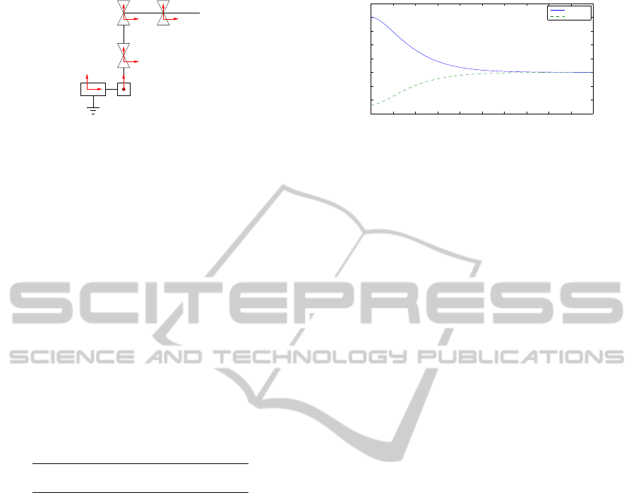
Figure 1: Kinematic representation of a mobile manipulator
5 DOF.
The actuators velocities, η ∈ R
4
, are defined as:
η = (v, ˙q
3
, ˙q
4
, ˙q
5
)
T
where v(t) is an scalar which describes the lineal ve-
locity of the mobile robot, and configuration kine-
matic model S(q) ∈ R
5×4
is defined by
S(q) =
cosq
3
0 0 0
sinq
3
0 0 0
0 1 0 0
0 0 1 0
0 0 0 1
(13)
which satisfy the property of being an annihilator for
(12). The parameters of (7) are obtained according to
(Spong et al., 2006) and the data that appears in Table
2.
Table 2: Link data for dynamic model from the 5-DOF mo-
bile manipulator.
i Length Wide Height Mass
[mm] [mm] [mm] [kg]
3 445 393 237 9.0
4 150 50 50 0.1
5 168 50 50 0.1
The control described in Section 4 was applied to
a numerical model of the mobile manipulator. The
result of the simulations are showed in Figure 2; the
reference is a trajectory in task space generated by a
linear interpolation between two points; it is impor-
tant to note that the trajectory not necessarily satisfy
the nonholonomic constraint.
6 CONCLUSIONS
This paper shows a systematic approach to model-
ing mobile manipulators that transforms the problem
to the modeling of a stationary manipulator station-
ary with non-holonomic kinematic constraints on the
joints. It is also presented a control that uses an esti-
mate of the derivative of the posture kinematic model.
Finally, an example is presented using this method.
In future work, it will develop a priority control in
the task space for a mobile manipulator, and it will be
develop a teleoperation scheme on the real system.
0 1 2 3 4 5 6 7 8 9 10
−0.15
−0.1
−0.05
0
0.05
0.1
0.15
0.2
0.25
Time [s]
Error [m]
Error on x
Error on y
Figure 2: Posture error graph for the mobile manipulator
under the control, as described in Section 4.
ACKNOWLEDGEMENTS
The authors appreciate the support of Mexican Gov-
ernment (SNI, SIP-IPN, COFAA-IPN, PIFI-IPN and
CONACYT).
REFERENCES
Bayle, B., Fourquet, J.-Y., and Renaud, M. (2003). Kine-
matic modelling of wheeled mobile manipulators. In
Robotics and Automation, 2003. Proceedings. ICRA
’03. IEEE International Conference on, pages 69–74.
Campion, G., Bastin, G., and Dandrea-Novel, B. (1996).
Structural properties and classification of kinematic
and dynamic models of wheeled mobile robots. IEEE
Trans. Robot., 12(1):47–62.
Corke, P. (1996). A robotics toolbox for MATLAB. IEEE
Robotics and Automation Magazine, 3(1):24–32.
De Luca, A. and Oriolo, G. (1995). Kinematics and Dy-
namics of Multi-Body Systems, chapter Modelling and
control of nonholonomic mechanical systems, pages
277–342. Springer.
De Luca, A., Oriolo, G., and Giordano, P. R. (2006). Kine-
matic modeling and redundancy resolution for non-
holonomic mobile manipulators. In Proceedings of
the 2006 IEEE International Conference on Robotics
and Automation, pages 1867–1873, Orlando, Florida,
USA.
Joshi, J. and Desrochers, A. (1986). Modeling and con-
trol of a mobile robot subject to disturbances. In Pro-
ceedings of the 1986 IEEE International Conference
on Robotics and Automation, pages 1508–1513.
Li, Y. and Liu, Y. (2004). Control of a mobile modular ma-
nipulator moving on a slope. In Mechatronics, 2004.
ICM ’04. Proceedings of the IEEE International Con-
ference on, pages 135–140.
Mazur, A. (2010). Trajectory tracking control in workspace-
defined tasks for nonholonomic mobile manipulators.
Robotica, 28:1–12.
Spong, M. W., Hutchinson, S., and Vidyasagar, M. (2006).
Robot Modeling and Control. Wiley.
Wang, Y., Lang, H., and de Silva, C. W. (2008). Visual servo
control and parameter calibration for mobile multi-
robot cooperative assembly tasks. In IEEE Interna-
tional Conference on Automation and Logistics, 2008.
ICAL 2008, pages 635–639, Qingdao.
ICINCO 2011 - 8th International Conference on Informatics in Control, Automation and Robotics
316
