CAUSAL REASONING IMPROVED BY FUZZY LOGIC

FOR DIAGNOSIS OF BOND GRAPH MODELLED

UNCERTAIN PARAMETERS SYSTEMS

Walid Bouallègue, Salma Bouslama Bouabdallah

LACS, National Engineering School of Tunis, BP 37, Le Belvedere, 1002, Tunis, Tunisia

Moncef Tagina

L3I, National School of Computer Sciences, Manouba, Tunisia

Keywords: Fault detection and isolation (FDI), Bond graph (BG), Parameters uncertainties, Fuzzy logic, Causal

reasoning.

Abstract: In this paper, a method for on-line fault detection and isolation (FDI) of bond graph (BG) modelled

uncertain parameters systems is proposed. In this case, we don’t have to calculate the Analytical

Redundancy Relations (RRAs) since residuals are directly generated from the Diagnostic Bond Graph

(DBG). Detection is based on fuzzy logic approach. For isolation, two methods exploiting the causal

properties of the BG model are used: Fault Signature Matrix (FSM), and exoneration. A real simulation

example is provided to show the efficiency of the proposed methods.

1 INTRODUCTION

Presently, Fault Detection and Isolation (FDI) is an

increasingly active research domain. FDI consists in

identifying when a fault has occurred, the type of

fault and its location. A widespread solution for FDI

consists in comparing the behaviour of the real

system to a theorical model.

FDI methods can be divided into three

categories: quantitative methods, qualitative

methods and process history based methods

(Staroswiecki, 2000); (Venkatasubramanian,

2003.a); (Venkatasubramanian, 2003.b); (Venkata-

subramanian, 2003.c).

The most frequently quantitative diagnosis

approaches are based on Analytical Redundancy

Relations (ARRs), Kalman filters and parameter

estimation. The ARRs are relations comparing

informations given by the real process to those

generated by the theorical model.

The qualitative methods are based on qualitative

models such as causal graphs, fault trees or

abstraction hierarchies … (Montmain and Gentil,

1999). These models are obtained by analyzing the

cause and effect relationships in the process and the

association of observations (symptoms) to failures

using qualitative operators.

Because of its behavioural, structural and causal

properties, the BG tool is used in complex processes

modelling and FDI (Samantaray and al., 2008);

(Dauphin-Tanguy, 2000); (Dauphin-Tanguy and

Tagina, 2000). Its causal properties are used to

determine the fault origins; Bond Graph is exploited

in both qualitative and quantitative diagnosis

methods (Samantaray et al., 2008).

Qualitative methods transform the BG model to a

qualitative model expressing the states of variables

with qualitative states ([+], [-] or 0) (Montmain and

Gentil, 1999). When an inconsistency (fault) is

detected, backward and forward propagation

procedure can be used for isolation. The BG model

can also be transformed to a Temporal Causal Graph

(TCG) or tree graph that can be used for FDI

(Samantaray et al., 2008).

In quantitative approaches, many methods are

proposed. By covering the causal paths in the BG

model, Analytical Redundancy Relations (ARRs)

can be derived from the energy conservation laws in

junctions 0 and 1, the principle of fault signature can

then be used to isolate the fault affecting sensors and

Bouallègue W., Bouslama Bouabdallah S. and Tagina M..

CAUSAL REASONING IMPROVED BY FUZZY LOGIC FOR DIAGNOSIS OF BOND GRAPH MODELLED UNCERTAIN PARAMETERS SYSTEMS.

DOI: 10.5220/0003537500590066

In Proceedings of the 8th International Conference on Informatics in Control, Automation and Robotics (ICINCO-2011), pages 59-66

ISBN: 978-989-8425-75-1

 2011 SCITEPRESS (Science and Technology Publications, Lda.)

actuators (Tagina, 1995). In (Samantaray et al.,

2006), residuals are directly generated in the

Diagnostic Bond Graph (DBG), and a fault signature

matrix (FSM) is elaborated by covering causal paths

from residuals detectors to the components.

Therefore, the efficiency and robustness of these

methods depend on the model’s accuracy.

In case of uncertain parameters systems, (Djeziri,

2007); (Djeziri et al., 2009) proposed a robust

diagnosis algorithm, from a BG model in Linear

Fractional Transformations (LFT) form. They

derived ARRs in which they separated the quantity

of energy given by the uncertain part from the

residual to be evaluated, this idea allows the

generation of adaptive thresholds for fault detection.

A study of sensitivity was elaborated to deduce

detectability indexes defining the detectable value of

the residual in case of faults and parameters

uncertainties. In (Bouallègue et al., 2010), a method

for robust fixed and adaptive thresholds is proposed.

This method exploits the sensitivity of residuals to

different system parameters in order to determine

their thresholds; the FSM is used for isolation. In

(Bouslama-Bouabdallah et al., 2006), a fuzzy logic

approach applied to residuals deduced from the BG

model is used in detection stage. For isolation, the

FSM is transformed into inference rules allowing the

determination of the fault’s origin.

The main contribution of this paper is to use the

bond graph model directly in the task of robust FDI

in case of uncertain parameters systems. The

detection module is based on a fuzzy logic system.

For isolation, two causal reasoning based methods

were proposed.

This paper is organized as follows: Section 2

details the notion of DBG used to generate directly

the residuals in the BG model. Section 3 describes

the proposed fuzzy detection method. Section 4

presents two isolation methods: signature matrix and

exoneration. Section 5 describes the hydraulic

benchmark composed of three tanks. Finally,

different results and their interpretations are given in

section 6.

2 RESIDUALS GENERATION

FROM DBG

The generation of Analytical Redundancy Relations

(ARRs) from the bond graph model uses the

structural relations given by the conservation law in

all 0 and 1 junctions and aims to express the

unknown variables by those known (inputs and

sensors). This method cannot deal with algebraic

loops, so, unknown variables cannot be eliminated.

So, the structural independence of the different

residuals has to be checked with existing residuals.

In (Samantaray et al., 2006), a direct method for

ARR generation from BG model is proposed. The

causality inversion of detectors (which are

considered as sources) has been proposed as a

unified approach to generate residuals.

When the bond graph model is assigned

preferred differential causality and using inversion

of sensor causalities, if necessary, the following five

compositions are possible (Samantaray et al., 2006):

1. Inverted causality in effort sensor (De),

2. Inverted causality in flow sensor (Df),

3. non-inverted causality in effort sensor (De),

4. non-inverted causality in flow sensor (Df),

5. Inversion of signal sensor, Ds, to signal

source, Ss (for controllers).

Let us consider the case of inverted causality in

the effort sensor, De, (see Figure 1). This sensor will

be equivalent to an effort source (measurements

from real process), so expression of the source

loading flow variable is equated to zero (Samantaray

et al., 2006). This expression is a residual (it does

not involve any states, since all storage elements are

in differential causality) which’s measured by a

virtual flow sensor (Samantaray et al., 2006).

Figure 1: (a) Sensor e in behavioral model, (b) inverted

causality in e and (c) substituted representation for

inverted causality in e.

The bond graph of the system with these

substitutions using preferred derivative causality is

called the Diagnostic Bond Graph (DBG)

(Samantaray et al., 2008).

3 DETECTION USING FUZZY

LOGIC APPROACH

In ideal conditions, residual value is equal to zero in

fault free context. In practice, due to the uncertainty

and the measurement noise, residuals are different

from zero. Thresholds are used to deduce whether

ICINCO 2011 - 8th International Conference on Informatics in Control, Automation and Robotics

systems are in normal functioning mode or faulty

mode. Unfortunately, thresholds near to zero can

cause false alarms problems because of noise

variation; and assigning larger thresholds reduce the

fault detection sensitivity (Frank et al., 1997).

Fuzzy logic is the most common solution to

overcome the uncertainty problems. Many works

used this approach in residuals processing in order to

know the system state (Evsukoff et al., 2000)

(Bouslama-Bouabdallah et al., 2006).

In this work, we propose fuzzy processing of

residuals generated by the DBG in the task of fault

detection in case of parameters uncertainty.

From residuals values, two features can be

extracted:

• The absolute value of the residuals: r

• Residual variation over a sliding time

window: d

dr(i)r(i)

+−

=−−

∑

The choice of the parameter N depends on the

residual variation and the noise effects, it is fixed

experimentally until we can get clearly the signal

trend.

The descriptor sets associated with each feature

fuzzy partition are:

r= {“SMALL”, “LARGE”}

d= {“SMALL”, “LARGE”}

These two variables are fuzzified using two

trapezoidal membership functions (Figure 2). So,

four parameters have to be determined for each

function.

Figure 2: Fuzzy sets of the residuals.

The trapezoidal boundaries of the set SMALL are

given by:

r : μ

small

=[0, 0, r-max, Rmin]

d : μ

small

=[0, 0, d-max, Dmin]

And for the set LARGE, they are given by:

r : μ

Large

=[r-max, Rmin, Rmax, Rmax]

d : μ

Large

=[d-max, Dmin, Dmax, Dmax]

Where:

r-max respectively d-max is the maximum value

of the residual respectively residual variation in

normal operating mode

Rmin = K

* r-max.

Dmin= K

*d-max ,

, K

is fixed experimentally.

Rmax respectively Dmax: is the maximum value

respectively variation of residual in faulty case.

For each residual, we have established a set of

inference rules which are presented in the following

table:

Table 1: Rules base of the fuzzy system.

Small Large

Small Normal Fault

Large Fault Fault

Rules are obtained using MIN-MAX inference

method, the MIN operator represents the logic

function AND, and the MAX operator for the logic

function OR.

The output of this fuzzy system is a fault index

indicating whether the concerned residual is in

normal operating mode or faulty mode (Figure 3).

Figure 3: Residual defuzzification.

4 THE PROPOSED FAULT

ISOLATION METHODS

Many procedures issued from FDI and Artificial

Intelligence communities were proposed in the task

of Fault Isolation. Causal properties of the BG tool

could be used in many methods such as Fault

Signature Matrix (FSM) and the exoneration

algorithm. In this work, these two methods are

combined with fuzzy reasoning in order to improve

FDI efficiency.

4.1 Signature Matrix

In FDI terminology, the Fault Signature Matrix

(FSM) crosses ARRs in rows and faults in column

(Cordier et al., 2004) (Biswas et al., 2009). Fault

isolation uses structural properties of the ARR

expressed in terms of a binary fault signature matrix

S, which describes the participation of various

CAUSAL REASONING IMPROVED BY FUZZY LOGIC FOR DIAGNOSIS OF BOND GRAPH MODELLED

UNCERTAIN PARAMETERS SYSTEMS

components (physical devices, sensors, actuators and

controllers) in each residual and forms a structure

that links the discrepancies in components to

changes in the residuals (Cordier et al., 2004).

Let us consider that fj is a fault affecting

component Cj, then in the binary fault signature

matrix F is,

, if the occurence of fault fj does not affect ARRi

, if the fault fj will violate ARRi

⎧

⎨

⎩

From the DBG model, the analysis of the causal

paths to each residual is used to generate these

signatures (Samantaray et al., 2006). In fact, every

component causally linked to the residual detector

can affect its value. Let us consider the DBG of

Figure 4:

Figure 4: Example of DBG.

If we consider residual detector r1, the next causal

paths can be found:

CÆf4Æf2Æf1Ær1

RÆf5Æf2Æf1Ær1

PÆe6Æe2Æe4ÆCÆf4Æf2Æf1Ær1

Then, any variation in components C, R and

sensor P can affect the value of residual r1. In the

same way, and using all residuals, we can deduce the

FSM.

In this work, fuzzy detection module output is

exploited in isolation task. So, a fuzzy fault

signature matrix F is defined as follows:

Small , if the occurence of fault fj does not affect ARRi

L arg e, if the fault fj will violate ARRi

⎧

⎨

⎩

4.2 Exoneration

4.2.1 Principle of Exoneration

Exoneration principle is a fundamental concept that

is often used implicitly in diagnosis (Cordier et al.,

2004); (Fagarasan et al., 2004). It uses consistency

of tests (residuals) to check if its support can be

faulty or not. The supports of a residual are variables

that can affect it and change its value. The

exoneration algorithm manages two lists, a list of

components whose state is normal, LN and a list of

suspect components LS. LS is made by the union of

the inconsistent test supports that are not exonerated

by the consistent tests (Fagarasan et al., 2004).

The steps of the algorithm are the followings

(Fagarasan et al., 2004):

1. Initialize L

and L

to the empty list 







={Ø}.

2. At each sampling time and for each test Ti:

2.1. IF Ti result is consistent, THEN Ti support Ci

is considered normal thus added to L

, L

={C

ᴗL

}

and deleted from L

, L

2.2. IF Ti result is inconsistent, Ti support Ci is

suspected of being faulty and its components that

are not in L

are added to L

={C

ᴗL

}\L

Finally, after the analysis of the tests, the

components in L

represent the final diagnosis.

4.2.2 Exoneration Improved by Fuzzy Logic

This algorithm is based on fuzzy logic to check the

consistency of the residuals. To use the fuzzy

detection module results, some improvements have

to be done.

1. Initialize L

and L

to the empty list 







={Ø}

2. At each sampling time and for each test Ti:

2.1. IF Ti result is NORMAL, then Ti

support Ci is considered normal thus added to

, L

={C

ᴗL

} and deleted from L

, L

2.2. IF Ti result is FAULT, then Ti support

Ci is suspected of being faulty and its

components that are not in L

are added to

={C

ᴗL

}\L

5 APPLICATION EXAMPLE

5.1 Test Bench Presentation

Let us consider the following hydraulic system

(Figure 5):

ICINCO 2011 - 8th International Conference on Informatics in Control, Automation and Robotics

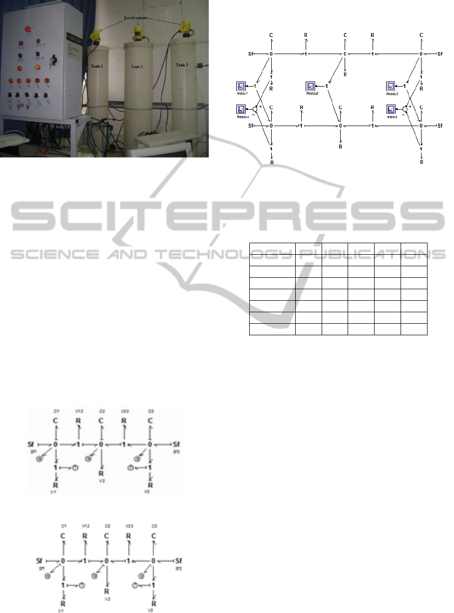
Figure 5: Real system.

This system is composed of three tanks T1, T2

and T3 respectively of diameters D1, D2 and D3;

water level in tanks, H1, H2 and H3 (proportional

respectively to the pressures P1, P2 and P3) is

measured by level sensors. This system is fed by two

pumps which deliver flows Sf1 (flow of entrance at

T1) and Sf2 (flow of entrance at T3).

Tanks T1 and T2 communicate through valve

V12 and tanks T2 and T3 through valve V23 of

diameter Sv. Each tank has a draining valve noted

Vi (i=1 to 3). Flow going out from valves V1 and

V2 is measured by flow sensors f1 and f2.

5.2 System BG Modelling

A procedure described in (Tagina, 1995) allows

elaborating the BG model of the system in integral

causality (Figure 6) as well as the corresponding

model in derivative causality (Figure 7).

Figure 6: BG model in preferred integral causality.

Figure 7: BG model in preferred differential causality.

The coupling between the two precedent models

produces the DBG of Figure 8:

Figure 8: DBG of the three tanks system.

From Figure 8, the following FSM can be

determined:

Table 2: Fault signature matrix of the three tanks system.

r1 r2 r3 r4 r5

Sf1 1 0 0 0 0

Sf2 0 0 1 0 0

V1 1 0 0 1 0

V12 1 1 0 0 0

V2 0 1 0 0 0

V23 0 1 1 0 0

V3 0 0 1 0 1

The supports of each residual deduced from the

DBG are given below:

:{Sf1, V1, V12}

:{V12, V2, V23}

:{Sf2, V23, V3}

:{V1}

:{V3}

6 EXPERIMENTAL RESULTS

6.1 Case of Normal Operating Mode

In Figure 9, different residuals in normal operating

mode are presented.

We notice that residuals have low values around

zero; this variation is due to parameters

uncertainties.

From Figure 9, we can deduce different

boundaries numeric values of the trapezoidal

memberships functions in the fuzzy detection

module. Different isolation methods were applied

with those boundaries. The results are given in

Figure 10. All the fault indexes of different methods

are equal to zero indicating that there are no faulty

CAUSAL REASONING IMPROVED BY FUZZY LOGIC FOR DIAGNOSIS OF BOND GRAPH MODELLED

UNCERTAIN PARAMETERS SYSTEMS

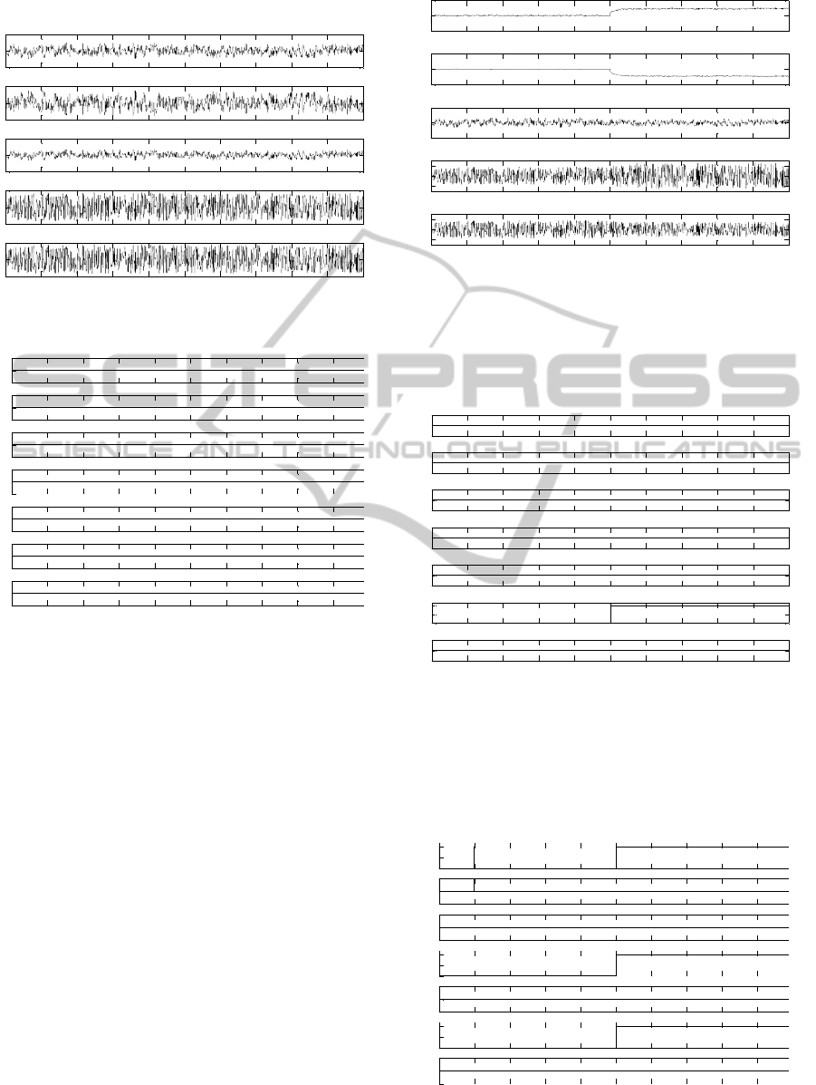
components.

Figure 9: Residuals evolution in normal operating mode.

Figure 10: Fault indexes with fault signature and

exoneration.

6.2 Case of Faulty Operating Mode

In case of faulty operating mode, some residuals

deviate from their normal values and isolation

methods are then used to identify the faulty

component.

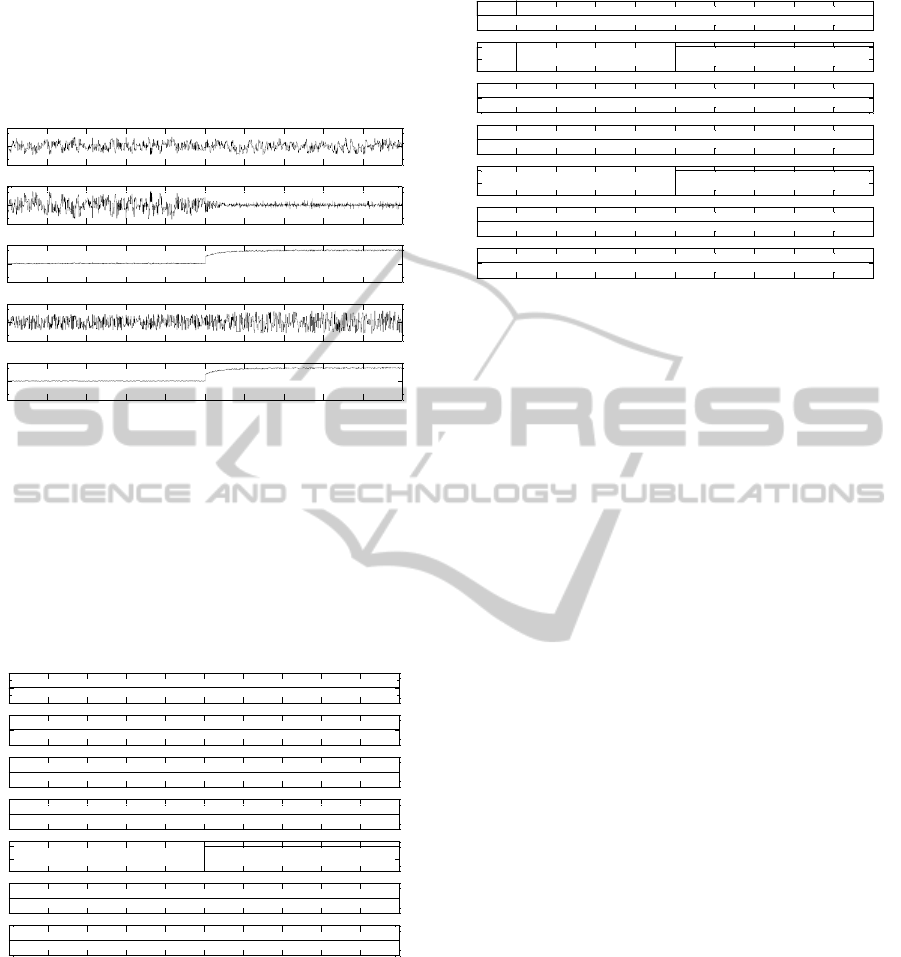
6.2.1 First Case: Fault affecting Valve V12

We totally fill in valve V12 at time 5000s; Figure 11

illustrates the evolution of the different residuals.

We notice, at the occurrence of the fault,

residuals sensors r1 and r2 deviation; all the other

residuals do not exceed normal functioning

thresholds, the signature (1, 1, 0, 0, 0) is equivalent

to fault in component V12 (Table 2).

Figure 12 represents the fault indexes generated

by the fuzzy FSM method. We notice that fault’s

origin is perfectly identified. In fact, fault index

DefR12 passes to 1 at instant 5000s.

Figure 11: Residuals evolution in case of V12 fault.

Figure 12 represents the fault indexes generated

by the fuzzy FSM method. We notice that fault’s

origin is perfectly identified. In fact, fault index

DefR12 passes to 1 at instant 5000s.

Figure 12: Fault indexes with fault signature matrix.

The results of localization by exoneration

algorithm are shown in Figure 13. In this case, the

fault indexes of components SF1, V2 and V12

passed to 1 at time 5000s. Then, we obtain 3

candidates components: {SF1, V2, V12}.

Figure 13: Fault indexes with exoneration algorithm.

0 1000 2000 3000 4000 5000 6000 7000 8000 9000 10000

-5

x 10

-5

Residuals variation

0 1000 2000 3000 4000 5000 6000 7000 8000 9000 10000

-1

x 10

-5

0 1000 2000 3000 4000 5000 6000 7000 8000 9000 10000

-5

x 10

-5

0 1000 2000 3000 4000 5000 6000 7000 8000 9000 10000

-1

x 10

-5

0 1000 2000 3000 4000 5000 6000 7000 8000 9000 10000

-1

x 10

-5

Time (s )

0 1000 2000 3000 4000 5000 6000 7000 8000 9000

-1

defSF1

Fault indexes

0 1000 2000 3000 4000 5000 6000 7000 8000 9000

-1

defSF2

0 1000 2000 3000 4000 5000 6000 7000 8000 9000

-1

defR1

0 1000 2000 3000 4000 5000 6000 7000 8000 9000

-1

defR2

0 1000 2000 3000 4000 5000 6000 7000 8000 9000

-1

defR3

0 1000 2000 3000 4000 5000 6000 7000 8000 9000

-1

defR12

0 1000 2000 3000 4000 5000 6000 7000 8000 9000

-1

defR23

Time(s)

0 1000 2000 3000 4000 5000 6000 7000 8000 9000 10000

-5

x 10

-4

Residuals' evolution

0 1000 2000 3000 4000 5000 6000 7000 8000 9000 10000

-5

x 10

-4

0 1000 2000 3000 4000 5000 6000 7000 8000 9000 10000

-5

x 10

-5

0 1000 2000 3000 4000 5000 6000 7000 8000 9000 10000

-1

x 10

-5

0 1000 2000 3000 4000 5000 6000 7000 8000 9000 10000

-1

x 10

-5

Time

(

)

0 1000 2000 3000 4000 5000 6000 7000 8000 9000 10000

-1

defSF1

Signature matrix

0 1000 2000 3000 4000 5000 6000 7000 8000 9000 10000

-1

defSF2

0 1000 2000 3000 4000 5000 6000 7000 8000 9000 10000

-1

defR1

0 1000 2000 3000 4000 5000 6000 7000 8000 9000 10000

-1

defR2

0 1000 2000 3000 4000 5000 6000 7000 8000 9000 10000

-1

defR3

0 1000 2000 3000 4000 5000 6000 7000 8000 9000 10000

0.5

defR12

0 1000 2000 3000 4000 5000 6000 7000 8000 9000 10000

-1

defR23

Time

(

)

0 1000 2000 3000 4000 5000 6000 7000 8000 9000

0.5

defSF1

Exoneration

0 1000 2000 3000 4000 5000 6000 7000 8000 9000

-1

defSF2

0 1000 2000 3000 4000 5000 6000 7000 8000 9000

-1

defR1

0 1000 2000 3000 4000 5000 6000 7000 8000 9000

0.5

defR2

0 1000 2000 3000 4000 5000 6000 7000 8000 9000

-1

defR3

0 1000 2000 3000 4000 5000 6000 7000 8000 9000

0.5

defR12

0 1000 2000 3000 4000 5000 6000 7000 8000 9000

-1

defR23

Time

(

)

ICINCO 2011 - 8th International Conference on Informatics in Control, Automation and Robotics

6.2.2 Second Case: Fault Affecting Valve V3

We suppose that valve V3 is closed at instant 5000s,

Figure 14 presents the evolution of the different

residuals in this case.

Figure 14: Residuals evolution in case of V3 fault.

We notice that residuals r3 and r5 are affected by

this fault and make a distinctive variation from their

normal values. The signature (0, 0, 1, 0, 1)

represents fault in component V3 (Table 2)

In Figure 15, fault indexes obtained by signature

matrix method are shown. This method localizes

perfectly the faulty component (V3).

Figure 15: Fault indexes with fault signature matrix.

Localization indexes determined by exoneration

procedure are given in Figure 16. They identify two

candidates to the fault: SF2 and V3.

Figure 16: Fault indexes with exoneration algorithm.

7 CONCLUSIONS

In this paper, fuzzy logic approach and causal

properties of the BG model are combined for FDI.

The residuals generated from the DBG are processed

in the fuzzy detection module. Output is a fault

index indicating whether the residual is faulty or it is

in fault free case.

Causal properties of the BG model allow using 2

localization methods: FSM and exoneration

algorithm. Our principle criterion to judge proposed

methods performances is the false alarm rate. The

FSM has proved its superiority in case of single fault

hypothesis. Exoneration methods give a conflict set

composed of more than one element in most cases.

REFERENCES

Biswas, G., Koutsoukos, X., Bregon, A., Pulido, B.

(2009). Analytic Redundancy, Possible Conflicts, and

TCG-based Fault Signature Diagnosis applied to

Nonlinear Dynamic Systems, Proceedings of the

IFAC-Safeprocess, Barcelona, Spain.

Bouallègue, W., Bouslama Bouabdallah, S., Tagina, M.

(2010). Diagnosis of Bond Graph modelled uncertain

parameters systems using residuals sensitivity,

Proceedings of the IEEE International conference on

Systems, Man, and Cybernetics, Turkey, 593-600.

Bouslama Bouabdallah, S., Tagina, M. (2006). A fuzzy

approach for fault detection and isolation of uncertain

parameter systems and comparison to binary logic,

IFAC, IEEE 3rd International Conference on

Informatics in Control, Automation and Robotics,

ICINCO 2006. Portugal, Intelligent Control Systems

and Optimization, 98-106.

Cordier, M. O., Dague, P., Dumas, M., Levy, F.,

Montmain, J., Staroswiecki, M., and Trave-Massuyes,

L. (2004). Conflicts versus Analytical Redundancy

0 1000 2000 3000 4000 5000 6000 7000 8000 9000 10000

-5

x 10

-5

Residuals' evolution

0 1000 2000 3000 4000 5000 6000 7000 8000 9000 10000

-1

x 10

-5

0 1000 2000 3000 4000 5000 6000 7000 8000 9000 10000

-5

x 10

-4

0 1000 2000 3000 4000 5000 6000 7000 8000 9000 10000

-2

x 10

-5

0 1000 2000 3000 4000 5000 6000 7000 8000 9000 10000

-5

x 10

-4

Time (s)

0 1000 2000 3000 4000 5000 6000 7000 8000 9000 10000

-1

defSF1

Signature matrix

0 1000 2000 3000 4000 5000 6000 7000 8000 9000 10000

-1

defSF2

0 1000 2000 3000 4000 5000 6000 7000 8000 9000 10000

-1

defR1

0 1000 2000 3000 4000 5000 6000 7000 8000 9000 10000

-1

defR2

0 1000 2000 3000 4000 5000 6000 7000 8000 9000 10000

0.5

defR3

0 1000 2000 3000 4000 5000 6000 7000 8000 9000 10000

-1

defR12

0 1000 2000 3000 4000 5000 6000 7000 8000 9000 10000

-1

defR23

Time (s)

0 1000 2000 3000 4000 5000 6000 7000 8000 9000 10000

-1

defSF1

Exoneration

0 1000 2000 3000 4000 5000 6000 7000 8000 9000 10000

0.5

defSF2

0 1000 2000 3000 4000 5000 6000 7000 8000 9000 10000

-1

defR1

0 1000 2000 3000 4000 5000 6000 7000 8000 9000 10000

-1

defR2

0 1000 2000 3000 4000 5000 6000 7000 8000 9000 10000

0.5

defR3

0 1000 2000 3000 4000 5000 6000 7000 8000 9000 10000

-1

defR12

0 1000 2000 3000 4000 5000 6000 7000 8000 9000 10000

-1

defR23

Time (s)

CAUSAL REASONING IMPROVED BY FUZZY LOGIC FOR DIAGNOSIS OF BOND GRAPH MODELLED

UNCERTAIN PARAMETERS SYSTEMS

Relations: a comparative analysis of the Model-based

Diagnosis approach from the Artificial Intelligence

and Automatic Control perspectives, IEEE Trans. on

Systems, Man, and Cybernetics (Part B), 34(5), 2163-

2177.

Dauphin-Tanguy, G. (2000). Les bond graphs, Hermès,

Paris.

Dauphin-Tanguy, G., Tagina, M. (2003). La méthodologie

bond graph: Principes et applications, Centre de

publications universitaires, Tunis.

Djeziri, M. A. (2007). Diagnostic des Systèmes Incertains

par l’Approche Bond Graph, Thesis, Ecole centrale of

Lille France.

Djeziri, M. A., Ould Bouamama, B., Merzouki, R. (2009).

Modelling and robust FDI of steam generator using

uncertain bond graph model, Journal of process

control.

Evsukoff A., Gentil S., Montmain J. (2000). Fuzzy

reasoning in co-operative supervision systems,

Control Engineering Practice, 389-407.

Frank, P. M., Köppen-Seliger. B. (1997). Fuzzy logic and

neural network applications to fault diagnosis,

International Journal of Approximate Reasoning,

Volume 16, Issue 1,67-88.

Fagarasan, I., Ploix, S., Gentil, S. (2004). Causal Fault

Detection and Isolation Based on a Set-Membership

Approach, Automatica, volume 40, 2099-2110.

Montmain, J., Gentil, S. (1999). Causal Modeling for

Supervision, Intelligent Control/Intelligent Systems

and Semiotics, Proceedings of the IEEE International

Symposium.

Samantaray A. K., Medjaher K., Ould Bouamama B.,

Staroswiecki M., Dauphin-Tanguy G. (2006).

Diagnostic bond graphs for online fault detection and

isolation. In Simulation Modelling Practice and

Theory.

Samantaray A. K., Ould Bouamama B. (2008). Model-

based Process Supervision: A Bond Graph Approach,

Springer.

Staroswiecki, M. (2000). Quantitative and qualitative

model for fault detection and isolation, Mechanical

Systems and Signal Processing, 2000.

Tagina, M. (1995). L'application de la modélisation bond

graph à la surveillance des systèmes complexes,

Thesis, University of Lille1, France 1995.

Venkatasubramanian, V., Rengaswamy, R., Kavuri, S. N.,

Yin, K. (2003.a). A review of process fault detection

and diagnosis Part I: Quantitative model-based

methods, Computers and Chemical Engineering 27,

293-311.

Venkatasubramanian, V., Rengaswamy, R., Kavuri, S. N.,

Yin, K. (2003.b). A review of process fault detection

and diagnosis Part II: Qualitative models and search

strategies, Computers and Chemical Engineering 27,

313-326.

Venkatasubramanian, V., Rengaswamy, R., Kavuri, S. N.,

Yin, K. (2003.c). A review of process fault detection

and diagnosis Part III: Process history based methods,

Computers and Chemical Engineering 27, 327-346.

ICINCO 2011 - 8th International Conference on Informatics in Control, Automation and Robotics