AutomationML AS A BASIS FOR OFFLINE

- AND REALTIME-SIMULATION -

Planning, Simulation and Diagnosis of Automation Systems

Olaf Graeser, Barath Kumar, Oliver Niggemann, Natalia Moriz and Alexander Maier

inIT-Institut Industrial IT, Hochschule Ostwestfalen-Lippe, Liebigstrasse 87, Lemgo, Germany

Keywords:

Automation technology, Modelling, Simulation, HIL test and AutomationML.

Abstract:

The growing complexity of production plants leads to a growing complexity of the corresponding automation

systems. Developers of such complex automation systems are faced with two signiﬁcant challenges: (i) The

control devices have to be tested before they are used in the plant. For this, ofﬂine- and hardware–in–the loop

(HIL) simulations can be used. (ii) The diagnosis functions within the automation systems become more and

more difﬁcult to implement; this entails the risk of undetected errors. Both challenges may be solved using a

system model, i.e. a joint model of the plant and the automation system: (i) Ofﬂine simulations and HIL tests

use such models as an environment model and (ii) diagnosis functions use such models to deﬁne the normal

system behaviour—allowing them to detect discrepancies between normal and observed behavior. System

models cannot be modelled by one person in a single development step. Instead, such models must mirror

the modularity of modern plants and automation systems. Here, the new standard AutomationML is used as

basis for such a modular system model. But a modular system model is only a ﬁrst step: Both testing and

diagnosis require the simulation of such models. Therefore, a corresponding modular simulation system for

AutomationML models is presented here; for this, the Functional Mock–Up Unit (FMU) standard is used. A

prototypical tool chain and a model factory (MF) is used to show results for this modular testing and diagnosis

approach.

1 INTRODUCTION

The virtual planning of factories (“Digital Factory”)

has been a major trend over the last years (see e.g.

(Brecher et al., 2008; K¨uhn, 2006)): By using sim-

ulated factories in early development phases, system

integrators and factory operators want to (i) minimise

design and construction times, (ii) reduce the num-

ber of errors in the factory and (iii) optimise factory

designs and conﬁgurations. This could lead to more

complex factories, faster processes, and more inte-

grated production chains.

So far, research in virtual factories has mainly fo-

cused on the plant and machine factory construction

aspect. But more complex factories also lead to more

complex automation systems. Here, we will present

a concept and ﬁrst prototypes for a modelling and

simulation approach for an automation-centred vir-

tual design and testing process. In other words, unlike

with machine-centred approaches, precise models of

the automation systems are used while the machines

and plants are only modelled with a limited level of

details—often timed event sequences are sufﬁcient.

A software tool chain for model based develop-

ment and simulation of a plant is introduced. This

tool chain starts with an editor for plant modelling and

ends in an simulation framework for ofﬂine simula-

tions, HIL tests and online plant diagnosis. These are

the three main use cases for the editor and the simu-

lation framework.

• In the ofﬂine simulation, Soft-PLCs (Pro-

grammable Logic Controllers), i.e. the control ap-

plications, can be tested by simulating Soft-PLCs

and the corresponding process.

• HIL tests can be used to test a PLC given as hard-

ware. Unlike an ofﬂine simulation, this requires a

real–time simulation.

• Online diagnosis can be used to detect changes

and anomalies in the behaviour of a plant—

mainly by comparing the real plant behaviorto the

simulated behaviour.

359

Graeser O., Kumar B., Niggemann O., Moriz N. and Maier A..

AutomationML AS A BASIS FOR OFFLINE - AND REALTIME-SIMULATION - Planning, Simulation and Diagnosis of Automation Systems.

DOI: 10.5220/0003537403590368

In Proceedings of the 8th International Conference on Informatics in Control, Automation and Robotics (ICINCO-2011), pages 359-368

ISBN: 978-989-8425-75-1

 2011 SCITEPRESS (Science and Technology Publications, Lda.)

2 STATE OF THE ART

For the automation technology, the challenge is to

model and develop control software, visualisation and

diagnosis software. Such software modules should be

reusable (for future projects), testable on a standalone

PC and platform independent(with respect to the used

communication hardware).

In the area of embedded systems software de-

velopment, several projects and standards addressed

the abovementioned challenges. For example safety–

related systems (IEC 61508, see (Gall, 2008)), auto-

motive software development (Steiner and Schmidt,

2003), the ﬁeld of automation (IEC 61499 and IEC

61131), or several research projects like Modale

(Szulman et al., 2005), OrVia (Stein et al., 2008) or

Medeia (Strasser et al., 2008).

The introduction of explicit systems, software and

plant models is an important trend in embedded soft-

ware development (Niggemann and Stroop, 2008;

Niggemann and Otterbach, 2008) and also in the

ﬁeld of automation technology (Szulman et al., 2005;

Strasser et al., 2008; Streitferdt et al., 2008). The

modelling approach in this work is based on control

and plant component models. For this purpose, stan-

dards like AutomationML (Drath et al., 2010) and

Modelica (Modelica Association, 2011) are used and

improved.

Furthermore, the concept of separation of con-

cerns is used. A complete plant model consists of var-

ious aspects, like logical software models, hardware

topologies, network descriptions and a system model.

For a better reusability of the single models, the mod-

els are modelled and stored separately. The combina-

tion of the single models is done in a later step. The

approach used in this work is inspired by the Object

Managements Group’s (OMG’s) Model–Driven Ar-

chitecture (MDA) (Allen, 2002; Mellor et al., 2004).

In the ﬁrst step, a logical structure with software mod-

ules and plant models is created. This correlates to

the MDA’s Platform IndependentModel (PIM). Later,

this structure is mapped onto speciﬁc hardware de-

scriptions. Components of the PIM, which describe a

class or a role of a device in the model, are thereby

linked to a real hardware. The result correlates then

to the MDA’s Platform Speciﬁc Model (PSM).

3 MODELLING

3.1 Concept

Factories and the corresponding automation systems

comprise more and more heterogeneous and inter-

connected components. Therefore the modelling for-

malism and the simulation framework must support

such systems. The new standard AutomationML

is able to integrate heterogeneous description for-

malisms and models automation systems, plants, sen-

sor/actuators, and especially their inter–connection.

Our modelling approach is in general inspired by

OMG’s MDA paradigm (see (Mellor et al., 2004) for

details): In a ﬁrst step, a logical architecture com-

prising only software modules and plant models is

created—MDA’s PIM. Only later on, this logical ar-

chitecture is mapped onto a speciﬁc hardware topol-

ogy, creating the system architecture—MDA’s PSM.

This can also be seen in ﬁgure 1.

Platform

Specific

Model

(PSM)

Platform

Independent

Model

(PIM)

Platform Model

(e.g. hardware

topology)

Transformation

and Mapping

Figure 1: Model Driven Architecture Approach.

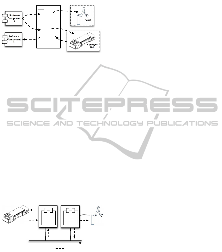
3.1.1 Platform Independent Model

As can also be seen in ﬁgure 2, PIMs comprise soft-

ware components (i.e. the software architecture) and

plant models. Software components are control al-

gorithms, diagnosis software algorithms, or monitor-

ing software modules. These software components do

not communicate directly with each other or with I/O

drivers but via plant signals. Plant signals are vari-

ables whose semantics are deﬁned by the plant model,

e.g. in ﬁgure 2 software component 1 sets the robot’s

”angle1” signal or start the conveyer belt by a ”start”

signal.

Please note, that plant signals usually correspond

to (physical) states of the real plant, i.e. unlike soft-

ware interfaces, they exist in reality and hence need

not be changed when the software architecture is

modiﬁed. This increases the level of software reuse

since software modules do not have to refer anymore

to software–speciﬁc interfaces. Since we only con-

ICINCO 2011 - 8th International Conference on Informatics in Control, Automation and Robotics

360

Robot

Plant Model

Software

Component

Software

Component

Conveyor

Belt

Plant Model

Plant

Roboter

Angle1

Angle2

Velocity

Conveyor Belt

Start

Velocity

Position

Packaging

Start

Plant Signals

Figure 2: Platform Independent Model.

sider automation systems, in most cases it is sufﬁcient

to restrict to the plant signals.

3.1.2 Platform Speciﬁc Model

PIMs have the advantage that they can be reused for a

large variety of hardware topologies (i.e. platforms).

For this, the PIMs are mapped in a second step onto

a speciﬁc hardware topology, creating a PSM. Many

features of the PSM can be derived automatically,

e.g. the schedule for real time communication net-

works such as I/O driver conﬁgurations or ProﬁNet

conﬁguration (see (PNO, 2007) for ProﬁNet details),

the scheduling algorithm is outlined in (Graeser and

Niggemann, 2009). This automatism allows develop-

ers to focus on the most difﬁcult part of the develop-

ment process: The development of the applications.

Such a PSM for the PIM from above can be seen

in ﬁgure 3: Software component 1 has been mapped

onto PLC 1, component 2 onto PLC 2. Now, unlike in

ﬁgure 2, the signal to start the conveyor belt must be

transmitted via the bus while the robot control signal

can be transmitted directly to the robot.

BUS

Software

Module

Robot

Start

Belt

Position

Start

Belt

Angle 1

Start

Belt

Start

Belt

PLC 1

PLC 2

Software

Module

Figure 3: Platform Speciﬁc Model.

Please note, that the same PIM can be mapped

onto a different hardware topology, i.e. this approach

leads to higher level of model reuse.

3.2 AutomationML System Model

As mentioned before, the key challenge lies in the

modelling and simulation of heterogeneous and mod-

ular systems; systems that comprise both the automa-

tion devices and the plants. As shownon the left–hand

side of ﬁgure 4, AutomationML is well suited for this

task, since the goal of AutomationML is to describe

a production plant completely, including all compo-

nents in it and to support each phase and discipline of

plant engineering. AutomationML is based on XML

and makes use of well established, open and free

XML based standards of the involved engineering

disciplines. For example, the object model is given

by CAEX (IEC 62424, 2008), geometries and kine-

matics are described by COLLADA (Khronos Group,

2011) and the behaviour of the plant is described with

PLCopen XML (PLCopen, 2011). Using these stan-

dards ensures a slim speciﬁcation of AutomationML

(Drath et al., 2010).

In AutomationML, a system is deﬁned as a hierar-

chy of inter–connected objects (bottom part of ﬁgure).

Each object may be the instance of a speciﬁc class

from a library—where a “RoleClass” deﬁnes an ab-

stract type such as a PLC and a “SystemUnitClass” a

speciﬁc product. From another point of view, a “Role-

Class” can be seen as requirements for an object, and

a “SystemUnitClass” is an implementation of these

requirements. Furthermore, objects communicate via

well–deﬁned interfaces.

Within the concept outlined here, interfaces were

deﬁned for plant modules, sensor/actuators, commu-

nication networks, and PLCs. These interfaces mainly

deﬁned incoming and outgoing signals and timing in-

formation.

AutomationML is able to include arbitrary XML

ﬁles. Here, an XML–based description of FMUs is

used to link objects in AutomationML to simulation

models. FMUs are a new standard from the Mod-

elisar project (Modelisar project, 2011) to provide

a uniform API to arbitrary simulations models such

as TheMathwork’s Simulink or Dassault’s Dymola.

In this project, a mapping between our interfaces in

AutomationML and FMU interfaces has been devel-

oped (right–hand side of ﬁgure 4). This allows for

mapping between AutomationML objects and FMU–

based simulation models, i.e. users are able to provide

heterogeneous simulation models for all our Automa-

tionML objects, hence supporting the required level

of support for heterogeneous and modular systems.

The interface to map FMUs to AutomationML ob-

jects is similar to all other external data mappings like

Collada and PCLopen XML. Both inherit from Au-

tomationML’s interface class “ExternalDataConnec-

tor”. Additionally to the “ColladaInterface” and the

“PLCOpenXMLInterface”, a “FMUInterface” is de-

ﬁned, which refers to an external FMU ﬁle. The in–

AutomationML AS A BASIS FOR OFFLINE - AND REALTIME-SIMULATION - Planning, Simulation and Diagnosis of

Automation Systems

361

AutomationML Library

Phoenix RFC 470, Siemens S7-200, ...

. . .

PLCs, Sensors, Networks, Plants

. . .

PLC Interface, Plant Interface, ...

. . .

Lemgoer Model Factory

PLC Central

Plant Modul 1

. . .

Interface

Modeling Simulation

Meta LevelInstance Level

Functional

Mockup

Unit (FMU)

Speciﬁcation

isOfType

Reference

Modelica

Model with

FMU

Interface

FMU 2

PLC

Model with

FMU

Interface

FMU 1

System Description in AutomationML

Figure 4: Modelling and simulating heterogeneous modular systems with AutomationML.

and output variables used in the FMU are described

in the “modelDescription.xml” inside the FMU ﬁle.

For now, the mapping to the variables in the Automa-

tionML format is done by name equality.

In this work, a drag and drop editor for a PIM as

described above was developed. The editor is based

on the Visual Studio 2010 Visualization and Model-

ing SDK (MSDN, 2011). The graphical user interface

can be seen in ﬁgure 6. Models created with this edi-

tor abstract from the communication hardware used in

the plant. As described above, software components

(e.g. PLC applications) are connected to sensors and

actuators via named signals.

The model of the plant is stored in Automa-

tionML format. Each component of the plant model

is mapped to an element of the AutomationML role

class lib. As mentioned before, the idea behind the

role class lib is, that each component in a plant has

to fulﬁl a function and has to play one or more roles.

Role classes can be understood, as a requirement def-

inition, which a component has to satisfy.

Using a graphical editor (Figure 6) has the advan-

tage over an XML editor, that new components (like

role classes) can be added to the model per drag–and–

drop and the relationships of the components and the

ﬂow directions of the communication signals are easy

to identify.

Using AutomationML increases the reusability of

the models, because it can be expected, that many

software tools in the ﬁeld of industrial automation

will at least support AutomationML im- and export.

Currently the plant is modelled only as PIM. Fu-

ture versions of the editor will also include the PIM to

PSM transformation. This can be done by assigning a

real hardware description to each AutomationML role

class lib based component of the PIM.

3.3 Modelica Behaviour Models

The behavioural model of the whole plant consists of

several sub–models, and is modular in nature. As

mentioned before in section (3), the plant signal in-

formation (i.e. incoming, outgoing signals and tim-

ing information) are often sufﬁcient enough to pro-

vide the necessary abstraction needed for modelling.

One possibility is to use Finite State Machine or

Automata (FSM) for constructing these behavioural

models. However, FSM do not support modeling

complex timed hybrid systems. Hence, our formalism

‘Probabilistic regression automata’ (PRA) described

in (Kumar et al., 2010a), which is an extension of

hybrid timed automata (Alur et al., 1995), (Sproston,

2000) is used for this purpose. In PRA, an event can

be triggered, when the value of one or several signals

cross the speciﬁed threshold value(s) within a cer-

tain time window reﬂecting the actual signal timing

of the real plant. In addition to the above, probabilis-

tic information is used to handle non-deterministic

scenarios (i.e. an automata can show different be-

haviours for the same set of inputs). A typical case

of non-determinism is occurrence of errors which is

inevitable (especially, in industrial automation sys-

tem) - however the occurrence of these errors is less

probable then the occurrence of the correct scenarios.

Moreover, our formalism supports continuous signals

and allows the arbitrary (not only linear) signal value

changes within a state.

ICINCO 2011 - 8th International Conference on Informatics in Control, Automation and Robotics

362

In this work, FSMs are implemented with Mod-

elica. Modelica is a free standardised equation–

based object–oriented modelling language. Modelica

is suitable for modular modelling of complex hetero-

geneous systems. By using Modelica, it is possible to

model signals with arbitrary complex behaviour,since

Modelica supports the hybrid DAEs (Differential Al-

gebraic Equations) systems. Modelica also supports

component–oriented modelling. This concept is con-

form with the concept of separation of concerns. This

also increases the reusability of single components of

the whole system. Moreover, single components can

be reﬁned as precisely as necessary.

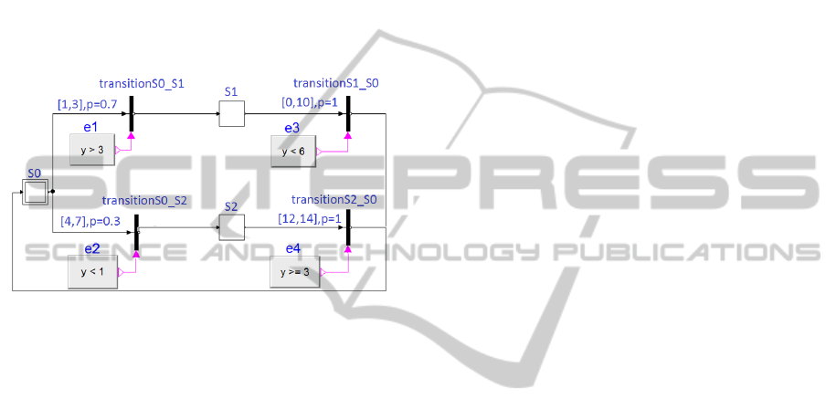
Figure 5: Finite state machine modelled with Dymola.

The automata used in this work were implemented

in Dymola (DASSAULT SYSTEMES, 2011). Dy-

mola is suitable for the requirements of modelling and

simulating production plants, because this tool sup-

ports hierarchical model composition, many libraries

of reusable components from several engineering do-

mains, faster simulation and open interfaces to other

programs (FMIs). Dymola enables users to develop

their own components. In our tool chain, the basis

for the PRA prototype is developed with the State-

Graph and StateGraph2 Modelica–standard libraries.

This basis is extended as following: (i) the interface

is added (the names of the variable are the same as

in the PLC program), (ii) the signal behaviour is in-

tegrated, (iii) the timing and probability information

is added. Currently our own library for PRA is un-

der development. An PRA prototype is represented in

ﬁgure 5.

Created behavioural models are stored as FMU.

FMUs are executables, which implemented the Func-

tional Mock–Up Interface (FMI). The FMI functions

are called by a simulator (here the ”FMU Simulation

Component”) to create and execute one or more in-

stances of the FMU. These FMUs can be referenced

in the abovementioned PIM-editor.

4 THE SIMULATION

FRAMEWORK

4.1 Simulation Framework

As mentioned before, the simulation framework

must support heterogeneous and inter–connected

components—mirroringAutomatioML’s capability to

model such systems. Here, a corresponding simula-

tion framework is described which uses the new stan-

dard FMU. This standard encapsulates heterogeneous

behaviour models such as Modelica or the Math-

work’s Simulink behind a standardised API.

The use cases of the project are ofﬂine simula-

tion for testing the control algorithms, HIL tests of

PLCs (and plant components), and anomaly detection

in the operating plant. For these use cases, a ﬂexi-

ble Simulation Framework was developed, in which

Simulation Components can be easily removed, re-

placed or added. The Simulation Framework consists

mainly of the Simulation Manager, which is responsi-

ble for the instantiation and scheduling of Simulation

Components, and the Process Data Manager, which

manages the process data of the plant model and dis-

tributes them to the Simulation Components (Figure

6).

The Simulation Framework makes use of the

Managed Extensibility Framework (MEF) (Mi-

crosoft, 2011) to connect all available Simulation

Components to the Simulation Framework. MEF is

part of Microsoft’s .NET frameworks and supports

the dynamic plug and play concept of software com-

ponents. Which Simulation Components are needed,

and in which quantity, is deﬁned in the Automa-

tionML plant description ﬁle coming from the Mod-

elling Tool (Section 3). The Simulation Components

are identiﬁed by theirs class name (e.g. ”FMU Sim-

ulation Component”). If more than one Simulation

Component of the same class is needed, additionally

a speciﬁc instance name is used.

The Process Data Manager is part of the Simula-

tion Manager. If a Simulation Component is instanti-

ated by the Simulation Manager, a process data input

list and an output list has to be registered at the pro-

cess data manager. The Process Data Manager then

compares the process data in the lists to the already

registered process data by name. New process data

will be added, already existing process data are linked

together (Figure 8).

4.2 Scheduling

One important task of the Simulation Manager is to

schedule all Simulation Components. For this pur-

AutomationML AS A BASIS FOR OFFLINE - AND REALTIME-SIMULATION - Planning, Simulation and Diagnosis of

Automation Systems

363

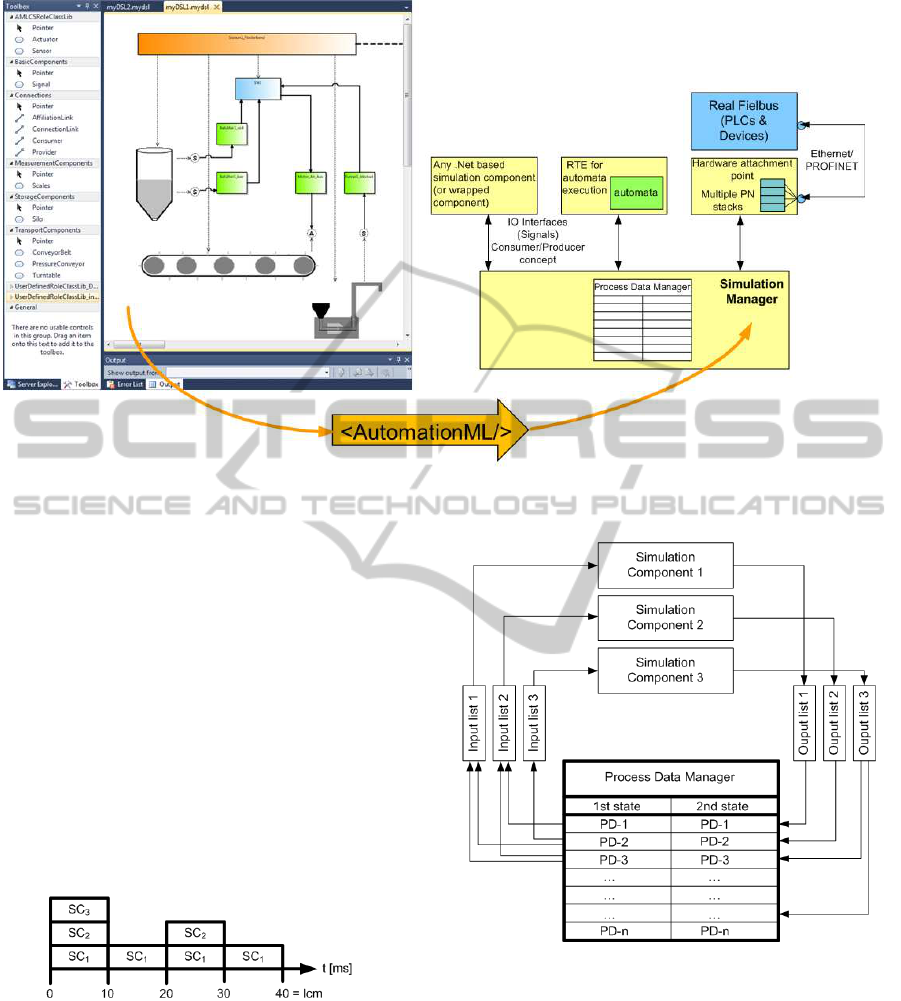
Figure 6: The PIM editor stores the plant model as AutomationML ﬁle. This ﬁle is then loaded into the Simulation Framework

to instantiate all needed Simulation Components.

pose a simple static scheduling algorithm is used. Ev-

ery Simulation Component has to declare, with what

time step the component needs to be scheduled. For

all these time steps, the least common multiple (LCM)

is calculated. Every Simulation Component is sched-

uled at the beginning (t

). Furthermore, each Simula-

tion Component is scheduled again with it’s speciﬁc

time step, as long as the time step sum is smaller than

the LCM. For example, in ﬁgure 7 three Simulation

Components (SC

, SC

) are scheduled. SC

with

a time step of 10ms, SC

with a time step of 20ms and

with a time step of 40ms. The LCM is therefore

40ms. The resulting schedule is cyclic, this means, as

soon as the end of the schedule is reached, the sched-

ule starts all over again.

Figure 7: Simulation Manager example schedule.

Currently, the Simulation Framework is not capa-

ble of parallel processing of Simulation Components.

Hence, the components are processed in sequence. It

is the responsibility of the Process Data Manager to

maintain two states of each process data (Figure 8).

The ﬁrst state contains the input process data of the

components. After the processing of a Simulation

Component, the resulting process data are written into

the second state.

Figure 8: The Process Data Manager.

After all parallel Simulation Components had

been processed, the resulting process data (second

state) are written into the ﬁrst state and are now avail-

able as input values for the next simulation step. Us-

ing this double buffer concept makes sure, that two or

more Simulation Components, which are scheduled at

the same time, work on the same set of process data.

4.3 Ofﬂine Simulation

For the ofﬂine simulation the AutomationML plant

ICINCO 2011 - 8th International Conference on Informatics in Control, Automation and Robotics

364

description ﬁle is loaded and all plant behaviour mod-

els, represented by FMUs, are loaded and instantiated

as FMU Simulation Components. Because the Simu-

lation Component ”FMU Simulation Component” is

used more than once, the instances have to be iden-

tiﬁed by theirs instance names, which can be given

by the ﬁle names of the loaded FMUs. After the cre-

ation of a schedule for all necessary simulation com-

ponents, the components are executed. The actual

process data in each time step are managed by the

Process Data Manager and can be logged by a spe-

cialised simulation component.

4.4 HIL Simulation

Hardware-In-the-Loop (HIL) is an approach to test

hardware devices such as PLCs or plant modules—

these devices are then called unit under test (UUT).

HIL differs from real–time or ofﬂine simulation by

considering the ‘actual’ device in the testing loop. In

a HIL test, a simulator (e.g. a special PC) simulates a

model of the environment for the attached UUT (i.e.

all other communicating partners of the overall sys-

tem, except the UUT); this can be seen in ﬁgure 9.

The purpose of HIL test is to make the UUT believe,

that it is in fact connected to the real system. By us-

ing a HIL test, UUTs can be tested with realistic plant

signals providing the necessary sensor/actuator trig-

gers to fully exercise the UUT — without requiring

the real system.

Hardware-in-the-Loop

Unit under

Test

Environment

Model

Figure 9: Hardware-in-the-Loop (HIL) Test Setup.

In automation, several parts of the overall system

may become the UUT; e.g. when several PLCs are

tested. Modular models as described in this paper, al-

low for a fast creation of the environment model by

removing those parts from the overall model that cor-

respond to the UUT.

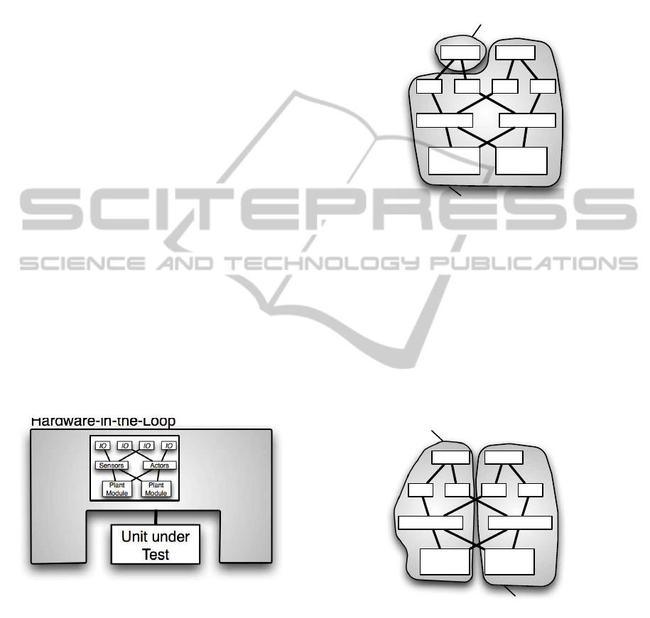
Figure 10 shows a typical HIL case in the do-

main of industrial automation: A real PLC is tested;

for this, the PLC model is removed from the over-

all model to create the environment model. The PLC

is then tested for correct responses, i.e. in terms of

(i) setting its actuator variables and (ii) performing its

duties meeting the real–time requirements of the over-

all system. The appropriate sensor inputs needed by

the PLC are sent at the right time by simulating the

environment model exploiting the input sample space

of the PLC under test.

PLC PLC

IO IO IO IO

Sensors Actors

Plant

Module

Plant

Module

Environment Model

Unit under Test (UUT) Model

Figure 10: Typical HIL case for automation.

Some typical errors in the automation domain for

which a PLC has to be tested are: (i) Functional in-

put space errors, i.e. does the PLC respond correctly

when a blocked funnel is sensed? and (ii) Time do-

main errors i.e. even if the PLC takes the right action;

Was it done within the required time limit? For e.g.

One such industrial automation test question covering

the above points would be: if the funnel is blocked

does the PLC stop the conveyor belt? - and does it do

it in time?

PLC PLC

IO IO IO IO

Sens./Act. Sens./Act.

Plant

Module

Plant

Module

Environment Model

Unit under Test (UUT) Model

Figure 11: Another typical HIL case for automation.

Another typical automation testing scenarios is

shown in ﬁgure 11: A whole plant module including

its PLC, IO devices, and the plant is being tested.

For testing, two key questions have to be solved:

(i) Where do the test cases come from? and (ii) Who

deﬁnes whether a test case was successful or failed—

this is the so–called test verdict. Generally speaking

two solution approaches exist:

1-Model-Approach. 1–Model–Approach considers

AutomationML AS A BASIS FOR OFFLINE - AND REALTIME-SIMULATION - Planning, Simulation and Diagnosis of

Automation Systems

365

one model for both test vector generation and code

generation for the UUT (e.g. PLC); the test verdict is

generated by comparing the test output with the pre-

diction of the UUT model. The key issue with this ap-

proach is: since the implementation and the test cases

are derived from the same model, only the code gen-

erator can be tested.

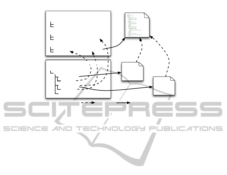
Figure 12: 2-Model-Approach.

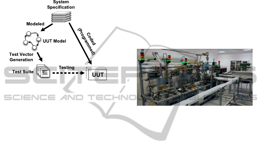
2-Model-Approach. 2-Model-Approach (also see

ﬁgure 12) on the other hand considers a separately im-

plemented unit under test (UUT), i.e. the UUT in pro-

grammed using conventional programminglanguages

(e.g. IEC 61131 languages, in case of PLC) based on

an existing informal speciﬁcation. In addition to this,

a speciﬁc formal testing model is developed based on

the same informal speciﬁcation and is used for test

vector generation; the test verdict is created by com-

paring the test output with the prediction of this test

model. Since the generated vectors and the UUT code

are not derived from the same model, this approach

provides the necessary redundancy needed for testing.

For our HIL test we use the 2-Model-Approach.

Our prototypical HIL test bed consists of a manu-

ally programmed (e.g. using IEC61131) UUT and the

testing model. The test model can be obtained in two

ways:

(i) by making use of the modular separation con-

cept of AutomationML (as shown in ﬁgure 10) - i.e.

in this case the environment model (overall model mi-

nus UUT model) is also the testing model. The simu-

lation framework can then be used to simulate all the

individual components (For e.g. other PLC models,

IOs and plant models, etc.) of the test model. Such

a testing scenario results in a closed loop test of the

UUT.

(ii) by generating test vectors from a single au-

tomaton which is obtained by merging the automata

of all the individual components of the environmen-

tal model. Such a test model can be used for an open

loop test.

In both of the above two scenarios, the test model

is used as a bases to extract ‘abstract test input se-

quences’ (our publication (Kumar et al., 2010b) de-

tails on the algorithmic concepts of test extraction)

either for simulating the environmental model (closed

loop) or for test execution (open loop). These ex-

tracted input sequences are ﬁrst serialized and then

built into appropriate industrial bus protocol frames

(in our case ProﬁNet IO frames). The HIL sends

these sensor values to the UUT (PLC) at appropriate

times, simulating the actual execution environment of

the UUT taking the real time requirements into con-

sideration. After the UUT reacts to these inputs, the

outputs are constantly monitored and compared with

the results predicted by the testing model.

Figure 13: A model factory.

Empirical Results. The HIL framework was used

for both closed loop and open loop tests for our ini-

tial test studies using a MF shown in ﬁgure 13. This

plant is used to produce and pack up bulk goods (e.g.

popcorn). This modular plant comprises of 8 mod-

ules, e.g. a storage system, several transportation

systems, a weighing mechanism, a bottling station, a

robot, a heating facility, and a packaging module. The

automation solution comprises of several distributed

PLCs to control the plants, buses such as ProﬁNet,

and approx. 250 sensor and actuator signals.

For the ﬁrst results, we performed open loop test

with just 2 modules of the MF. To test the credibility

of the generated test vectors - 24 mutants (16 func-

tional (i.e. actuator errors) and 8 timing errors) were

introduced into the PLC control logic, which were

positively identiﬁed. A test model for closed loop test

with 2 modules of the MF were modelled using Mod-

elica FMUs; these FMUs were simulated using the

proposed simulation framework to imitate the execu-

tion environment of the PLC. Further, tests were con-

ducted for ideal plant scenarios and with 4 functional

and 2 timing errors; which were correctly detected by

the HIL framework. Table 1 summaries HIL test’s ini-

tial results. Even though, the ﬁrst results are positive -

further studies are needed to check complex test sce-

narios; For e.g. including all 8 modules of the MF and

by including error with an exhaustive exploitation of

mutant sample space.

ICINCO 2011 - 8th International Conference on Informatics in Control, Automation and Robotics

366

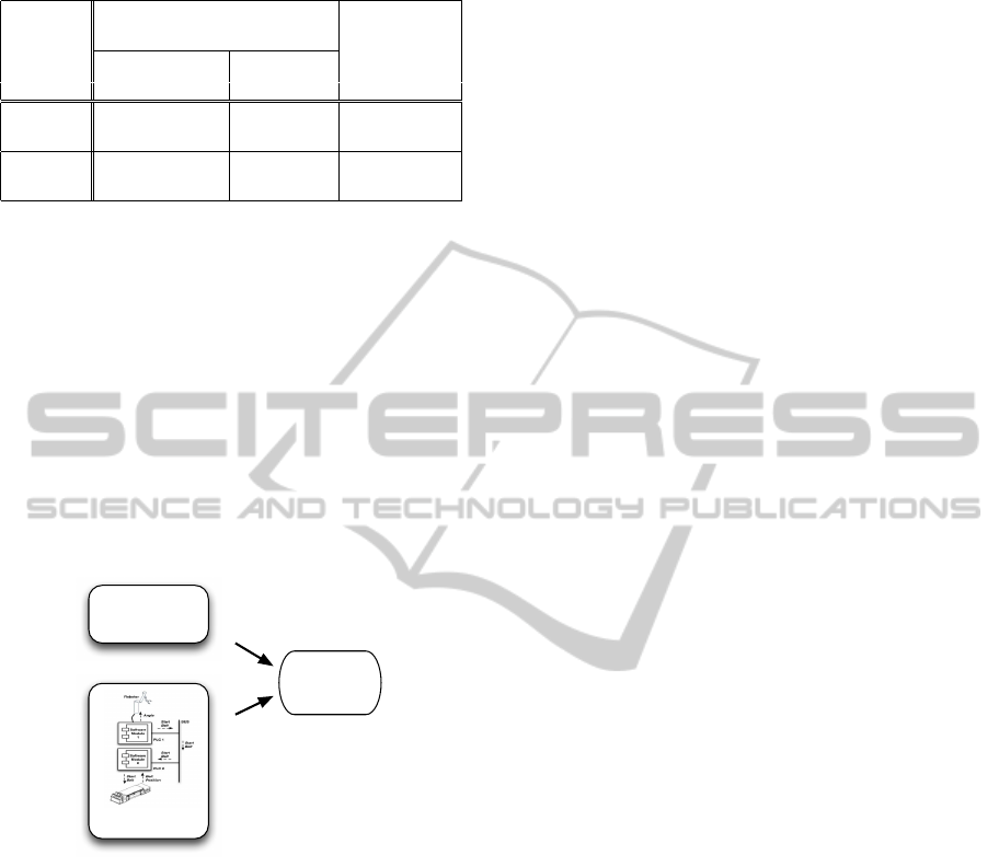
Table 1: HIL test results.

Type of Test

Inserted mutants

Detected mutants

Functional mutants Timed mutants

Closed Loop 4 2 6

Open Loop 16 8 24

4.5 Anomaly Detection

The detection of system deterioration and of non–

normal system behaviour will prove essential for the

improvement of system quality and reliability: Pro-

duction facilities could detect failures earlier and in-

spections can be planned whenever ﬁrst sign of dete-

rioration appears.

The key idea is rather simple: Let M be a sys-

tem model which captures all fault relevant system

aspects; here we use the model from section 3. When-

ever M’s behaviour shows a discrepancy to the sys-

tem’s current behaviour, the user will be alarmed.

Discrepancy

Detection

System Model

System

Measurements

Simulation

Figure 14: Detection of system deterioration.

This can also be seen in ﬁgure 14: During the run-

time of the system, the simulations of the model M

are constantly compared to the system behaviour and

discrepancies are detected.

Generally speaking, the ofﬂine simulation from

section 4 can be used for the anomaly detection.

There are three main differences. The ﬁrst one is, that

the simulation is slowed down, so that the clock in the

simulation matches the clock of the real world com-

munication system. The second difference is, that a

specialised simulation component is used, which is

able to read all process data (inclusive time stamps)

from a real plant. The third difference is, that the sim-

ulated process data and the real world process data are

compared in every single simulation step. The idea is,

that if the simulated process data are different to the

real world process data, an anomaly is supposed to be

detected (compare (Supavatanakul et al., 2006)).

This approach is currently tested for the appli-

cation of anomaly detection: The predictions of the

model are compared to measurements from the real

plant; if a discrepancy occurs, an anomaly is sig-

nalled. For this, the MF discussed in section 4.4 is

used.

For a ﬁrst veriﬁcation of the approach, we only use

3 of the plant modules and we deﬁne 3 types of errors:

a blocked sensor, a sensor communication error, and a

deteriorationeffects of a conveyer belt. Then, for each

of the 4 cases (3 errors, one OK case), we recorded 30

production cycles and tried to detect the errors. All

errors have been identiﬁed correctly.

5 CONCLUSIONS

Even though the development of the PIM editor and

the Simulation Framework is still in progress, this

software tool chain already enables a user to create an

abstract and modular PIM model of a productionplant

and to store it in an AutomationML based ﬁle for-

mat. AutomationML is well suited for this purpose,

because of its hierarchical CAEX structure and its ex-

tendable interface concept. These interfaces are cur-

rently used to describe the behaviour of the individual

components in the plant model by state automatons

as (self executing) FMUs, but the modular concept of

Simulation Components also allows for different ap-

proaches.

The usage of the FMI is at the moment a neces-

sary requirement to execute these automatons in the

Simulation Framework. The Simulation Framework

reads the required communication connections from

the AutomationML plant model and instantiates all

needed Simulation Components with the correspond-

ing in- and output lists of process data. The process

data then are managed by the Process Data Manager,

which enables the individual Simulation Components

to communicate among each other, and which pro-

vides them with the process data appropriate to the

clock of the corresponding components.

For a demonstration purpose, this tool chain al-

ready had been used for the ofﬂine simulation of a

production plant, a HIL test of a single component (a

PLC) and for the anomaly detection (diagnosis) in an

operating production plant. Future work will extend

the PIM editor with the functionality of mapping real

hardware to the model. As a result, the editor will be

a PIM/PSM editor then.

AutomationML AS A BASIS FOR OFFLINE - AND REALTIME-SIMULATION - Planning, Simulation and Diagnosis of

Automation Systems

367

REFERENCES

Allen, P., editor (2002). The OMG’s Model Driven Architec-

ture, volume XII of Component Development Strate-

gies, The Monthly Newsletter fromthe Cutter Informa-

tion Corp. on Managing and Developing Component-

Based Systems.

Alur, R., Courcoubetis, C., Halbwachs, N., Henzinger,

T. A., Ho, P.-H., Nicollin, X., Olivero, A., Sifakis, J.,

and Yovine, S. (1995). The algorithmic analysis of

hybrid systems. THEORETICAL COMPUTER SCI-

ENCE, 138:3–34.

Brecher, C., Fedrowitz, C., Herfs, W., Kahmen, A., Lohse,

W., Rathjen, O., and Vitr, M. (2008). Durchg¨angiges

Production Engineering Potenziale der digitalen Fab-

rik. In Brecher, C., Schmitt, F. K. R., and Schuh,

G., editors, Wettbewerbsfaktor Produktionstechnik:

Aachener Perspektiven. Aachen AWK.

DASSAULT SYSTEMES (2011). Dymola. http://

www.dymola.com.

Drath, R., Weidemann, D., Lips, S., Hundt, L., L¨uder, A.,

and Schleipen, M. (2010). Datenaustausch in der An-

lagenplanung mit AutomationML. Springer.

Gall, H. (2008). Functional safety IEC 61508 / IEC 61511

the impact to certiﬁcation and the user. In AICCSA

’08: Proceedings of the 2008 IEEE/ACS Interna-

tional Conference on Computer Systems and Applica-

tions, pages 1027–1031, Washington, DC, USA. IEEE

Computer Society.

Graeser, O. and Niggemann, O. (2009). Planung

der

Ubertragung von Echtzeitnachrichten in Netzw-

erken mit Bandbreitenreservierung am Beispiel von

Proﬁnet IRT. In Echtzeit 2009 - Software-intensive

verteilte Echtzeitsysteme GI-Fachauschuss, Boppard,

Germany.

IEC 62424 (2008). Festlegung f¨ur die Darstellung von Auf-

gaben der Prozessleittechnik in Fliessbildern und f¨ur

den Datenaustausch zwischen EDV-Werkzeugen zur

Fliessbilderstellung und CAE-Systemen.

Khronos Group (2011). Collada - 3d asset exchange

schema. http://www.khronos.org/collada/.

K¨uhn, W. (2006). Digital factory: simulation enhancing

the product and production engineering process. In

WSC ’06: Proceedings of the 38th conference on Win-

ter simulation, pages 1899–1906. Winter Simulation

Conference.

Kumar, B., Niggemann, O., and Jasperneite, J. (2010a).

Statistical models of network trafﬁc. In International

Conference on Computer, Electrical and Systems Sci-

ence.

Kumar, B., Niggemann, O., and Jasperneite, J. (2010b).

Test generation for hybrid, probabilistic control mod-

els. In Entwurf komplexer Automatisierungssysteme

(EKA 2010). Magdeburg, Germany.

Mellor, S., Scott, K., Uhl, A., and Weise, D. (2004). MDA

Distilled: Principles of Model-Driven Architecture.

Addison Wesley.

Microsoft (2011). Managed extensibility framework.

http://mef.codeplex.com/.

Modelica Association (2011). Modelica. https://

www.modelica.org/.

Modelisar project (2011). Functional mock-up interface.

http://functional-mockup-interface.org/.

MSDN (2011). Visual studio visualization and modeling

sdk. http://code.msdn.microsoft.com/vsvmsdk.

Niggemann, O. and Otterbach, R. (2008). Durchge-

hende Systemveriﬁkation im Automotiven Entwick-

lungsprozess. In Tagungsband des Dagstuhl-

Workshops Modellbasierte Entwicklung eingebetteter

Systeme IV (MBEES), Schloss Dagstuhl, Germany.

Niggemann, O. and Stroop, J. (2008). Models for model’s

sake: why explicit system models are also an end

to themselves. In ICSE ’08: Proceedings of the

30th international conference on Software engineer-

ing, pages 561–570, New York, NY, USA. ACM.

PLCopen (2011). http://www.plcopen.org/.

PNO (2007). Proﬁnet speciﬁcation iec 61158-5-10 (v2.1).

Sproston, J. (2000). Decidable model checking of proba-

bilistic hybrid automata.

Stein, S., K¨uhne, S., Drawehn, J., Feja, S., and Rotzoll, W.

(2008). Evaluation of OrViA Framework for Model-

Driven SOA Implementations: An Industrial Case

Study. In 6th International Conference on Business

Process Management, Milan, Italy.

Steiner, P. and Schmidt, F. (2003). Anforderungen und

Architektur zuk¨unftiger Karosserieelektroniksysteme.

In VDI Berichte Nr. 1789.

Strasser, T., Sunder, C., and Valentini, A. (2008). Model-

driven embedded systems design environment for the

industrial automation sector. In Proceedings of the

6th IEEE International Conference on Industrial In-

formatics, Daejeon, South Korea.

Streitferdt, D., Wendt, G., Nenninger, P., Nyssen, A., and

Lichter, H. (2008). Model driven development chal-

lenges in the automation domain. In Computer Soft-

ware and Applications, 2008. COMPSAC ’08. 32nd

Annual IEEE International, pages 1372–1375.

Supavatanakul, P., Lunze, J., Puig, V., and Quevedo, J.

(2006). Diagnosis of timed automata: Theory and

application to the damadics actuator benchmark prob-

lem. Control Engineering Practice, 14(6):609–619.

Szulman, P., Assmann, D., Doerr, J., Eisenbarth, M., Hefke,

M., Soto, M., and Trifu, A. (2005). Using ontology-

based reference models in digital production engi-

neering integration. In Proceedings of the 16th IFAC

WORLD CONGRESS, Prague.

ICINCO 2011 - 8th International Conference on Informatics in Control, Automation and Robotics

368