
OPTIMUM TRAJECTORY PLANNING FOR INDUSTRIAL
ROBOTS THROUGH INVERSE DYNAMICS
K. Koray Ayten, P. Iravani and M. Necip Sahinkaya
Department of Mechanical Engineering, University of Bath, BA2 7AY, Bath, U.K.
Keywords: Optimum control, Inverse dynamics, Torque minimization, Trajectory planning.
Abstract: This paper presents a method for developing robot trajectories that achieve minimum energy consumption
for a point-to-point motion under kinematic and dynamic constraints. The method represents trajectories as
a fourth degree B-spline function. The parameters of the function are optimised using a multi-parametric
optimization algorithm. Actuator torques have been considered for the formulation of the cost function,
which utilizes an inverse dynamics analysis. Compared to other trajectory optimization techniques, the
proposed method allows kinematic and dynamic constraints to be included in the cost function. Thus, the
complexity and computational effort of the optimization algorithm is reduced. A two-link simulated robot
manipulator is used to demonstrate the effectiveness of the method.
1 INTRODUCTION
Most of industrial robotic applications are based on
repetitive processes, where minimum cycle time is
an important factor to reduce the production time
and to increase the profit of the production (Zoller
and Zentan, 1999). However, the minimum time
criterion is not suitable if a smooth path for the
motion is required. When the actuators run at high-
speeds, they can cause physical vibrations and
undesirable shocks to the system. These unwanted
vibrations can result in a wide range of problems
including loss of accuracy, increased energy
consumption and a decrease in actuator life.
Energy requirement has been a significant
feature in robotic systems, e.g. robots for space or
submarine exploration, or unmanned reconnaissance
vehicles (Saravanan and Ramabalan, 2008). This
paper focuses on energy minimization in the context
of trajectory planning. The cost function in
(Gasparetto and Zanotto, 2007) and (Zanotto and
Gasparetto, 2007) consists of two terms. The first
term is the total execution time and the second is the
jerk. Some of the approaches include the travel time
in the cost function (LoBianco and Piazzi, 2002).
Also the mechanical power of the actuators and
energy for gripper action are considered for the
formulation of cost function in (Saramago and
Ceccarelli, 2004) and just the mechanical power in
(Garg and Kumar, 2002).
This paper proposes a path planning trajectory
method to generate an optimum path based on
minimum torque and/or energy consumption. The
proposed method considers an inverse dynamic
model of the robot manipulator. The resulting
optimization algorithm can be applied to various
robots, such as redundant or parallel robots in order
to optimize the desired trajectory. The method has
the advantage that kinematic and dynamic
constraints are included in a sequential manner in
the cost function and solving the inverse dynamics is
avoided when the constraints are not satisfied.
In this study, the dynamic modelling of the robot
is based on Lagrangian dynamics (Wells, 1967),
which describes the system in terms of its energy.
The DYSIM software (Sahinkaya, 2004) is used to
construct the equations of motion automatically for
both forwards and inverse dynamic analysis of the
system. In this study, DYSIM was operated in the
MatLab/Simulink.
2 OPTIMIZATION
Path planning techniques are associated with the
way in which a robot manipulator moves from one
point to another in a controlled manner (Niku,
2001). One of the important stages of path planning
is that of trajectory optimization. Trajectory
optimization problems can be divided into the
105
Ayten K., Iravani P. and Sahinkaya M..
OPTIMUM TRAJECTORY PLANNING FOR INDUSTRIAL ROBOTS THROUGH INVERSE DYNAMICS.
DOI: 10.5220/0003536301050110
In Proceedings of the 8th International Conference on Informatics in Control, Automation and Robotics (ICINCO-2011), pages 105-110
ISBN: 978-989-8425-74-4
Copyright
c
2011 SCITEPRESS (Science and Technology Publications, Lda.)

following components:
• Parametric path function
• Path coordinates
• Optimization technique
• Cost function
• Constraints
2.1 Parametric Path Function
Selection of the parametric path function is the first
step of the trajectory optimization technique.
Generally in optimization, a small number of
parameters is preferred without restricting the
motion space. Also, for manipulator motions, the
trajectory function has to be at least twice
differentiable in order to provide smooth and
continuous accelerations.
In this study, a fourth order B-spline function is
used to define joint motions because of its simplicity
and computational efficiency (De Boor, 1978), see
(Qin, 2000) for details. A fourth order B-spline
function consists of nine parameters. Three of them
are used for the start condition (position, and its first
and second derivatives). Three parameters are used
for the end condition (position, and its first and
second derivatives). The remaining three free
parameters are calculated by the optimization
algorithm.
2.2 Path Coordinates
Trajectory planning can be done either in the joint-
space or Cartesian-space. Planning a trajectory in the
joint-space has a significant advantage that the
control system will be acting on the robot joints
rather than on the end effector. In this case, it is
easier to set the necessary trajectory in terms of the
design requirements. However, the trajectory of the
end effectors will not be easily predictable (Niku,
2001). On the other hand, Cartesian-space
trajectories are more realistic and very simple to
visualize, but these have to be converted to joint
space for control purposes. In this paper, joint space
trajectories are used. However, the method can
handle Cartesian-space trajectories if required.
2.3 Optimization Technique
The selection of the optimization technique is
important as a large number of parameters and
coefficients may adversely affect the results of
optimization, and computational efficiency (Garg
and Kumar, 2002). In the proposed method, there is
no need to use computationally intensive
optimization techniques such as genetic algorithms.
Therefore, a sequential quadratic programming
technique (the default method in""
function in MatLab (The Mathworks, 2007) is used.
2.4 Cost Function
In the literature, the most common objectives to be
optimized are minimum travelling time, minimum
energy (or actuator effort, e.g. torque), and minimum
jerk (Gasparetto and Zanotto, 2007).
Minimum energy consumption was taken into
account here, but other quantitative indicators could
be considered according to design objectives. The
cost function of actuator effort (or torque)
minimization is described by:
=
()
(1)
where is the actuator cost function,
the actuator
torques/forces applied at joint along the trajectory,
K the number of actuators, and the total travelling
time between initial and final positions. Calculation
of the cost function in Eq. (1) requires the solving of
the inverse dynamic model for T seconds. Three free
parameters of the B-spline function are used to
optimize each joint trajectory.
2.5 System Constraints
Robot manipulators will have some physical
constraints such as the limits of the position,
velocity, acceleration and torque. Using these
constraints, unrealistic or unreachable motions of the
manipulator are automatically avoided in the
optimization procedure. Other constraints can also
be added (such as obstacle avoidance, singularity
avoidance) to the optimization algorithm for
trajectory planning.
The cost function calculations involve running
the inverse dynamic model, which is time
consuming. In conventional methods the constraint
equations are handled separately, and the cost
function is called regardless of whether the
constraints are satisfied or not. In order to improve
computational efficiency in the proposed method,
constraints are handled within the cost function
calculations and the inverse dynamic analysis is only
evaluated when these constraints are satisfied. In
order to achieve this, an alternative cost function is
formulated to handle constraints as follow:
1. A variable, c, is created to count the number of
cost function calls where the parameters do
ICINCO 2011 - 8th International Conference on Informatics in Control, Automation and Robotics
106
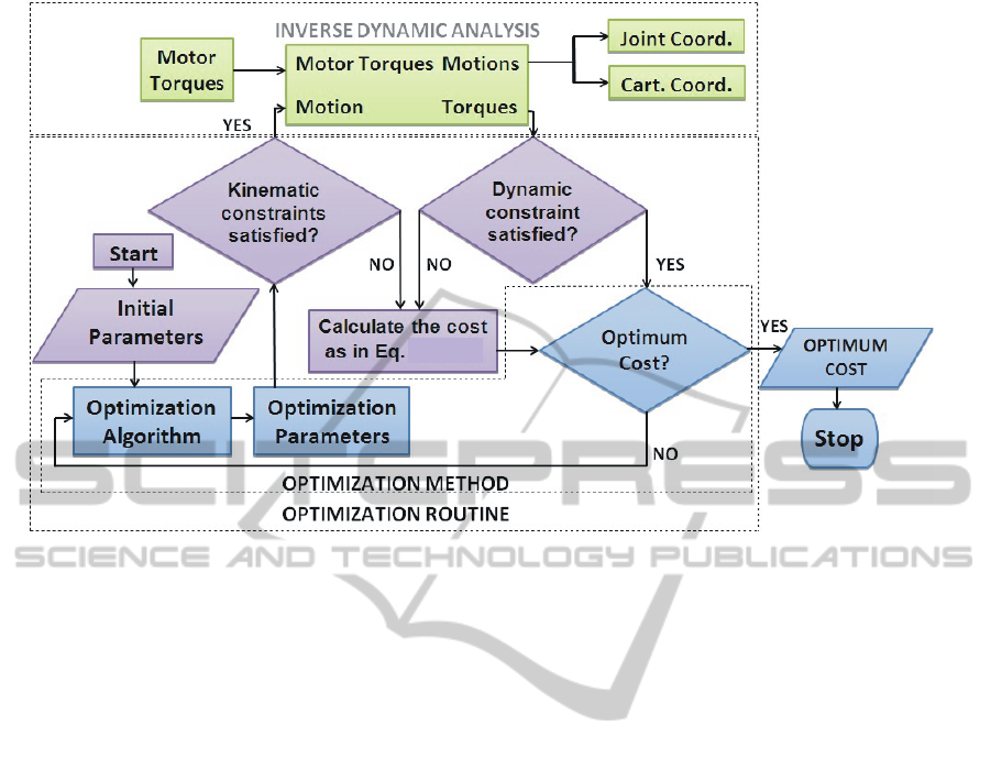
Figure 1: Optimization routine with inverse dynamic programming.
not satisfy the constraint equations.
2. During the cost function call, if any of the
constraints are not satisfied, the following
alternative cost function is used:
=+1 (2)
=∗(1+/10) (3)
where b is a large base value. This formulation
ensures that the cost function will result in a higher
value than previous violation of constraints to avoid
a local minimum to be found outside the constraints.
The value b=10
5
is used here.
3 PROPOSED ALGORITHM
The steps of the proposed energy minimization
algorithm based on inverse dynamics analysis can be
summarized as follow:
1. Before executing the optimization algorithm, all
kinematic and dynamic constraints of the
mechanism have to be identified. In this
example, constraints are based on maximum and
minimum values of position, velocity,
acceleration and torque.
2. Thereafter, the optimization algorithm will start
with suitable initial conditions in joint
coordinates.
3. When calculating the cost function, the
optimization algorithm will check the kinematic
constraints.
a) If the kinematic constraints are not satisfied,
the inverse dynamic analysis will not be carried
out. The alternative calculation of the cost
function will be carried out in accordance with
Eqs. (2) and (3).
b) If the kinematic constraints are satisfied,
inverse dynamic simulation will be run in order
to calculate the dynamic cost function as in Eq.
(1). If the torque limitations or other dynamic
constraints are violated, the simulation will be
terminated and the alternative cost function in
3 (a) above will be used.
4. This procedure will continue until the
optimization algorithm finds the lowest cost
value. The procedure of the optimization
algorithm is shown in Fig 1.
4 SYSTEM DESCRIPTION AND
SIMULATION
This section introduces numerical simulations using
a simple 2-DOF planar manipulator with revolute
joints as shown in Fig. 2. The simulation is carried
out by the program DYSIM. Two motors control the
motion. The centre of gravity of the links is in the
middle of the each link. A load mass of
= 1 kg is
(2,3)
OPTIMUM TRAJECTORY PLANNING FOR INDUSTRIAL ROBOTS THROUGH INVERSE DYNAMICS
107
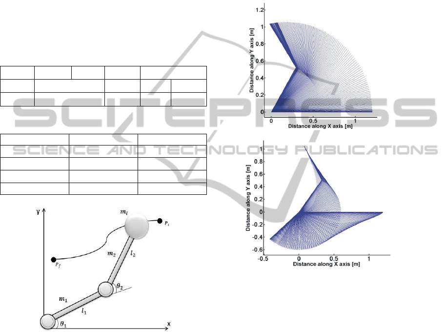
attached at the end of the second link. The
manipulator has two identical links detailed in Table
1. Gears ratios are
=100,
=80. The viscous
friction effects of the joints are also included in the
simulation.
The manipulator task consists of transporting the
load mass from an initial point
(
=
=0)
to a final one
(
=
=1) in joint space
coordinates. The motion duration is specified as
T=2s. The initial and final velocities and
accelerations are zero for all joints. The limits for
each actuator are given in Table 2.
Table 1: 2-DOF robot manipulator data.
Joints Length Mass Inertia Friction
Joint 1
0.6
1
0.01 0.4
Joint 2
0.6
1
0.01 0.4
Table 2: Limit performances of the 2-DOF manipulator.
Conditions Joint 1 Joint 2
()() -/+3/2 -/+3/2
()(/)
-/+6 -/+6
()(/
)
-/+25 -/+25
()()
-15/+25 -15/+25
Figure 2: Schematic diagram of the robot and a prescribed
trajectory given by initial and final points.
5 RESULTS AND DISCUSSION
The proposed method was implemented in Simulink.
The prescribed non-optimized (initial) manipulative
task is shown in temporal trajectory position in Fig.
3(a), and the optimum trajectory is traced in Fig.
3(b). The labels ‘−’ and
‘’ in the figures denote the result for the
case with initial parameter values corresponding to a
linear motion in joint space and the case with
optimization, respectively.
Figure 4 shows profiles of joint position (),
velocity (/), torque () and cost function
results. The initial path was a straight line in the
joint space between
and
and cost value for the
non-optimized trajectory was 897.683. After
optimization, the cost function is reduced to
620.129, which corresponds to 31% energy
consumption reduction.
Figure 3: Temporal positions of (a) non-optimized and (b)
optimized trajectories.
Figure 4(b) shows that optimized velocity is
faster than the non-optimized one. As it can be seen
from the Fig. 4(c), non-optimized link-1 has a large
peak torque magnitude. Figure 4(d) shows the
evolution of the cost functions. There is a sudden
ascension on the non-optimized cost curve.
Excessive growth of the cost value can be shown to
be due to lifting of the first and second arm with
minimum joint movements between 0 and 0.5
seconds. On the other hand, optimized cost curve is
increasing smoothly by utilising the potential energy
of the system.
The optimization was also run by using different
friction coefficient values. Temporal position results
are shown in Fig. 5. With increasing coefficient of
viscous friction in the system, the trajectory of the
end effectors has noticeable changed. The trajectory
(a)(a)
(b)
ICINCO 2011 - 8th International Conference on Informatics in Control, Automation and Robotics
108
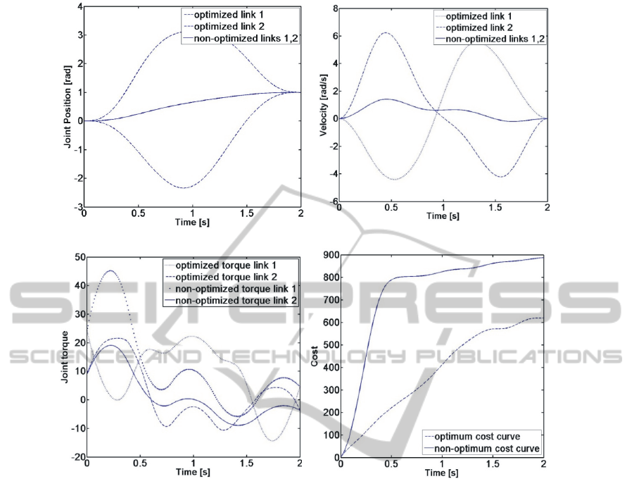
Figure 4: Results for the designed non-optimal and optimal path in terms of time history of (a) joint positions, (b) joint
velocities, (c) joint torques, and (d) cost value of the system.
of the end effector moves towards minimum joint
displacements in order to minimize energy
consumption in the system.
Each cost function call (whether within the
workspace or not) requires the inverse dynamic
simulations, which has significant effect on the
computational efficiency of the optimization. The
computational cost in the proposed algorithm is
reduced due to not running the inverse model in the
alternative cost function calculations when the
constraints are not satisfied. To further demonstrate
the advantages of the proposed algorithm over the
conventional method of handling the constraints, the
same optimization was run with Mathlab “fmincon”
function with the cost function as in Eq. (1), and the
constraints specified separately as nonlinear
inequality constraints. It was observed that the
optimization algorithm called the cost function even
when the parameters did not satisfy the constraints.
The number of cost function calls with parameters
values outside the permissible workspace was
significant (82 out of 243 iterations), resulting
unnecessary solving of the inverse dynamics.
In addition to computational efficiency, in cases
where the B-splines are used to describe the
trajectory in Cartesian coordinates, an additional
nonlinear constraint has to be added to make sure
that the end point does not fall outside the circle of
radius
21
ll +
during the motion. The conventional
constraint handling would still call the inverse
dynamics model when this constraints was not
satisfied. This would cause the inverse dynamics
simulation to crash or terminate prematurely as the
required motion cannot be physically achieved. The
proposed algorithm avoids this problem.
6 CONCLUSIONS
A methodology for optimal trajectory planning of
robotic manipulators has been described in this
(b)
(a)
(d)
(c)
OPTIMUM TRAJECTORY PLANNING FOR INDUSTRIAL ROBOTS THROUGH INVERSE DYNAMICS
109
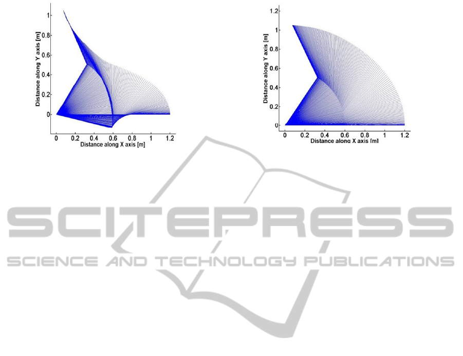
(a) friction coefficient of 1.5 (b) friction coefficient of 5
Figure 5: Results for the designed optimal path in terms of temporal positions for increasing friction values.
paper. A fourth degree B-spline function was used to
define the trajectory and hence the continuity of
velocity and accelerations were guaranteed for the
desired trajectory. An inverse dynamic analysis of a
two degree of freedom manipulator is performed by
using Lagrangian dynamics and an in-house
software package Dysim. In the proposed
optimization method, all the constraints are built in
the cost function. Therefore, computational
complexity is reduced by avoiding inverse dynamic
analysis when the parameters produce a motion that
does not satisfy the constraints. The proposed
algorithm also avoids the problems with cases where
the inverse dynamics model cannot be run when
some specific constraints are not satisfied.
REFERENCES
De Boor, C., 1978. A Practical Guide to Spline, Springer.
New York.
Garg, D, P., Kumar, M., 2002. Optimisation techniques
applied to multiple manipulators for path planning and
torque minimisation. Engng Appl Artif Intell 15, pp.
241–252.
Gasparetto, A., Zanotto, V., 2007. A technique for time-
jerk optimal planning of robot trajectories. Robotics
and Computer-Integrated Manufacturing. In:
press:doi:10.1016/j.rcim.
LoBianco, C, G., Piazzi, A., 2002. Minimum-time
trajectory planning of mechanical manipulators under
dynamic constraints. Int J Contr 75 (13), pp. 967–980.
Niku, S, B., 2001. Introduction to Robotics: Analysis,
Systems, Applications, Prentice Hall.
Qin, K., 2000. General Matrix Representations for B-
Splines. Visual Computer, vol. 16, no. 3/4, pp. 177-
186.
Sahinkaya, M, N., 2004. Inverse dynamic analysis of
multiphysics systems. Proceedings of the Institution of
Mechanical Engineers Part 1-Journal of System and
Control Engineering. 218(T1): 13-26.
Saramago, S., Ceccarelli, M., 2004. Effect of basic
numerical parameters on a path planning of robots
taking into account actuating energy. Mechanical and
Machine Theory 39, pp. 247–260.
Saravanan, R., Ramabalan, S., 2008. Evolutionary
minimum cost trajectory planning for industrial robots.
Journal of Intelligent and Robotic Systems 52:1, pp.
45-77.
The Mathworks Inc. Matlab R2007a. Computer Program.
Wells, Dare, A., 1967. Schaum's Outline of Theory and
Problems of Lagrangian Dynamics with a treatment of
Euler's Equations of Motion, Hamilton's Equations,
and Hamilton's Principle. New York: McGraw Hill
Book Company.
Zanotto, V., Gasparetto, A., 2007. A new method for
smooth trajectory planning of robot manipulators.
Mech Machine Theory, 42, pp. 455–471.
Zoller, Z., Zentan, P., 1999. Constant Kinetic Energy
Robot Trajectory Planning. Peridica Polytechnicaser.
Mech. Eng. Vol. 43, No.2, 213 – 228.
ICINCO 2011 - 8th International Conference on Informatics in Control, Automation and Robotics
110
