
INNER AND OUTER CAPTURE BASIN APPROXIMATION WITH
SUPPORT VECTOR MACHINES
Laetitia Chapel
Lab-STICC, Universit
´
e Europ
´
eenne de Bretagne, Universit
´
e de Bretagne Sud, 56017 Vannes Cedex, France
Guillaume Deffuant
Laboratoire d’Ingnierie pour les Syst
`
emes Complexes, Cemagref, 63172 Aubi
`
ere Cedex, France
Keywords:
Viability theory, Capture basin, Optimal control, Support Vector Machines.
Abstract:
We propose a new approach to solve target hitting problems, that iteratively approximates capture basins at
successive times, using a machine learning algorithm trained on points of a grid with boolean labels. We
consider two variants of the approximation (from inside and from outside), and we state the conditions on the
machine learning procedure that guarantee the convergence of the approximations towards the actual capture
basin when the resolution of the grid decreases to 0. Moreover, we define a control procedure which uses the
set of capture basin approximations to drive a point into the target. When using the inner approximation, the
procedure guarantees to hit the target, and when the resolution of the grid tends to 0, the controller tends to
the optimal one (minimizing time to hit the target). We use Support Vector Machines as a particular learning
method, because they provide parsimonious approximations, from which one can derive fast and efficient
controllers. We illustrate the method on two simple examples, Zermelo and car on the hill problems.
1 INTRODUCTION
We focus on the problem of defining the control func-
tion for driving a dynamical system to reach a given
target compact set C ⊂ K in minimum time, without
going out from K, where K is a given set (called con-
straint set). This problem, often called the reacha-
bility problem, can be addressed by optimal control
methods, solving Hamilton-Jacobi-Bellman (HJB) or
Isaacs (HJI) equations. Several numerical techniques
are available; for example, (Mitchell et al., 2005) pro-
pose an algorithm that computes an approximation for
the backward reachable set of a system using a time
dependent HJI partial differential equation, (Lygeros,
2004) builds the value function of the problem which
can be then used to choose the best action at each time
step.
Reachability problem can also be addressed in the
viability theory framework (Aubin, 1991). To ap-
ply viability theory to target hitting problems, one
must add an auxiliary dimension to the system, rep-
resenting the time elapsed before reaching the tar-
get. The approach computes an approximation of the
envelopes of all t-capture basins, the sets of points
for which there exists a control function that allows
the system to reach the target in a time less than t.
(Frankowska, 1989) shows that the boundary of this
set is the value function in the dynamical program-
ming perspective. Hence, solving this extended via-
bility problem also provides the minimal time for a
state x to reach the target C while always staying in
K (minimal time function ϑ
K
C
(x) (Cardaliaguet et al.,
1998)). This function can then be used to define con-
trollers that drive the system into the target.
Several numerical algorithms (Saint-Pierre, 1994;
Cardaliaguet et al., 1998) provide an overapproxima-
tion of capture basins. (Bayen et al., 2002) imple-
ment an algorithm proposed by (Saint-Pierre, 2001)
that computes a discrete underapproximation of con-
tinuous minimal time functions (and thus an overap-
proximation of capture basins), without adding an ad-
ditional dimension. (Lhommeau et al., 2007) present
an algorithm, based on interval analysis, that provides
an inner and outer approximation of the capture basin.
In general, capture basin and minimal time function
approximation algorithms face the curse of dimen-
sionality, which limits their use to problems of low
dimension (in the state and control space).
This paper proposes a new method to solve tar-
get hitting problems, inspired by our work on via-
34
Chapel L. and Deffuant G..
INNER AND OUTER CAPTURE BASIN APPROXIMATION WITH SUPPORT VECTOR MACHINES.
DOI: 10.5220/0003536000340040
In Proceedings of the 8th International Conference on Informatics in Control, Automation and Robotics (ICINCO-2011), pages 34-40
ISBN: 978-989-8425-74-4
Copyright
c
2011 SCITEPRESS (Science and Technology Publications, Lda.)

bility kernel approximation (Deffuant et al., 2007).
The principle is to approximate iteratively the cap-
ture basins at successive times t. To compute time
t-capture basin approximation, we use a discrete grid
of points covering set K, and label +1 the points for
which there exists a control leading the point into the
t −δt-capture basin approximation, and -1 otherwise.
Then, we use a machine learning method to compute
a continuous boundary between +1 and -1 points of
the grid. We state the conditions the learning method
should fulfil (they are similar to the one established to
approximate viability kernels (Deffuant et al., 2007))
in order to prove the convergence toward the actual
capture basins.
We consider two variants of the algorithm: one
provides an approximation that converges from out-
side, and the other from inside. Although no conver-
gence rate is provided, the comparison of the two ap-
proximations gives an assessment of the approxima-
tion error for a given problem. Moreover, we define
a controller that guarantees to reach the target when
derived from the inner approximation.
We consider Support Vector Machines (SVMs
(Vapnik, 1995; Scholkopf and Smola, 2002)) as a rel-
evant machine learning technique in this context. In-
deed, SVMs provide parsimonious approximations of
capture basins, that allow the definition of compact
controllers. Moreover, they make possible to use op-
timisation techniques to find the controls, hence prob-
lems with control spaces in more dimensions become
tractable. We can also more easily compute the con-
trol on several time steps, which improves the quality
of the solution for a given resolution of the grid.
We illustrate our approach with some experiments
on two simple examples. Finally, we draw some per-
spectives.
2 PROBLEM DEFINITION
We consider a controlled dynamical system in dis-
crete time (Euler approximation), described by the
evolution of its state variable x ∈ K ⊂ R
n
. We would
like to define the set of controls to apply to the sys-
tem starting from point x in order to reach the target
C ⊂ K in minimal time:
(
x(t + dt) = x(t) + ϕ(x(t),u(t)).dt, if x(t) /∈ C
x(t + dt) = x(t), if x(t) ∈ C
u(t) ∈ U,
(1)
where ϕ is a continuous and derivable function of x
and u. The control u must be chosen at each time step
in the set U of admissible controls.
The capture basin of the system is the set of states
for which there exists at least one series of controls
such that the system reaches the target in finite time,
without leaving K. Let G(x,(u
1
,..,u
n
)) be the point
reached when applying successively during n time
steps the controls (u
1
,..,u
n
), starting from point x. Let
the minimal time function (or hitting time function) be
the function that associates to a state x ∈ K the mini-
mum time to reach C:
ϑ
K
C
(x) = inf
{
n|∃(u
1
,..,u
n
) ∈ U
n
such that G(x, (u
1
,..,u
n
)) ∈ C
and for 1 ≤ j ≤ n,G (x,(u
1
,..,u
j
)) ∈ K
.
(2)
This is the value function obtained when solving HJB
equations in a dynamic programming approach. It
takes values in N
+
∪ +∞, specifically ϑ
K
C
(x) = 0 if
x ∈ C and ϑ
K
C
(x) = +∞ if no trajectory included in K
can reach C. The capture basin of C viable in K is
then defined as:
Capt(K, C) =
n
x ∈ K|ϑ
K
C
(x) < +∞
o
, (3)
and we can also define the capture basin in finite time
n:
Capt(K, C,n) =
n
x ∈ K|ϑ
K
C
(x) ≤ n
o
. (4)
To solve a target hitting problem in the viability per-
spective, one must consider the following extended
dynamical system (x(t),y(t)) when x(t) /∈ C:
x(t + dt) = x(t) + ϕ(x(t), u(t)) .dt
y(t + dt) = y(t) − dt.
(5)
and (x(t + dt) = x(t),y(t + dt) = y(t)) when x(t) ∈ C.
(Cardaliaguet et al., 1998) prove that approximating
minimal time function comes down to a viability ker-
nel approximation problem of this extended dynam-
ical problem. In a viability problem, one must find
the rule of controls for keeping a system indefinitely
within a constraint set. (Bayen et al., 2002; Saint-
Pierre, 2001) give examples of such an application of
viability approach to solve a target hitting problem.
(Deffuant et al., 2007) proposed an algorithm,
based on (Saint-Pierre, 1994), that uses a machine
learning procedure to approximate viability kernels.
The main advantage of this algorithm is that it pro-
vides continuous approximations that enable to find
the controls with standard optimization techniques,
and then to tackle problems with control in large di-
mensional space. The aim of this paper is to adapt
(Deffuant et al., 2007) to compute directly an approx-
imation of the capture basin limits, without adding the
auxiliary dimension, and then to use these approxima-
tions to define the sequence of controls.
INNER AND OUTER CAPTURE BASIN APPROXIMATION WITH SUPPORT VECTOR MACHINES
35

3 MACHINE LEARNING
APPROXIMATION OF VALUE
FUNCTION CONTOURS AND
OPTIMAL CONTROL
For simplicity, we denote Capt(K, C,n.dt) = Capt
n
.
In all the following, continuous sets are denoted by
rounded letters and discrete sets in capital letters.
We consider function G:
G(x,u) =
x + ϕ(x,u).dt if x /∈ C
x if x ∈ C
(6)
We suppose that G is µ-lipschitz with respect to x:
∀(x,y) ∈ K
2
,∀u ∈ U|G(x,u) − G(y, u)| < µ|x − y|.
(7)
We define a grid K
h
as a discrete subset of K, such
that:
∀x ∈ K,∃x
h
∈ K
h
such that |x − x
h
| ≤ h. (8)
Moreover, we define an algebraic distance d
a
(x,∂E)of
a point x to the boundary ∂E of a continuous closed set
E, as the distance to the boundary when x is located
inside E, and this distance negated when x is located
outside E:
if x ∈ E, d
a
(x,∂E) = d(x,∂E), (9)
if x /∈ E, d
a
(x,∂E) = −d(x,∂E). (10)
3.1 Capture Basin Approximation
Algorithms
In this section, we describe two variants of an algo-
rithm that provides an approximation C
n
h
of the cap-
ture basin at time n.dt, one variant approximates the
capture basins from outside and the other one from
inside. At each step n of the algorithm, we first build
a discrete approximation C
n
h
⊂ K
h
of the capture basin
Capt
n
, and then we use a learning procedure L (for in-
stance Support Vector Machines, as shown below) to
generalise this discrete set into a continuous one C
n
h
:
C
n
h
= L(C
n
h
) (11)
To simplifying the writing, we first define:
C
n
h
=
{
x
h
∈ K
h
s.t. x
h
/∈ C
n
h
}
, (12)
C
n
h
=
{
x ∈ K s.t. x /∈ C
n
h
}
. (13)
The two variants differ on the conditions for defining
the discrete set C
n+1
h
from C
n
h
, and on the conditions
the learning procedure L must fulfil. For both variant,
we construct an increasing sequence of approxima-
tions at time n.dt, by adding the points of the grid for
which there exists at least one control that drives the
system not too far away (in an algebraic sense - nega-
tive distance in the outer case and positive distance in
the inner one) from the boundary of the previous ap-
proximation. They also both require conditions on the
learning procedure, in order to guarantee the conver-
gence toward the actual capture basin when the step
of the grid h decreases to 0. In the inner approxima-
tion case, the condition is stricter on set C
n
h
and more
relaxed on set C
n
h
, while the outer case requires con-
verse conditions. We now describe in more details
both variants and conditions.
3.1.1 Outer Approximation
Given initial sets C
0
h
= C ∩ K
h
, C
0
h
= C, and supposing
that we define continuous approximations C
n
h
from C
n
h
(eq. (11)), we define discrete sets C
n
h
as follows:
C
n+1
h
= C
n
h
S
x
h
∈ C
n
h
s.t. ∃u ∈ U,
d
a
(G(x
h
,u),∂C
n
h
) ≥ −µh
.
(14)
Proposition. If the learning procedure L respects the
following conditions:
∀x ∈ C
n
h
,∃x
h
∈ C
n
h
s.t. |x − x
h
| ≤ h (15)
∃λ ≥ 1s.t.∀h,∀x ∈ C
n
h
,∃x
h
∈ C
n
h
s.t. |x − x
h
| ≤ λh (16)
then the convergence of the approximation from out-
side is guaranteed:
∀n,Capt
n
⊂ C
n
h
, (17)
C
n
h
→ Capt
n
when h → 0. (18)
Proof. The proof is given on appendix 5.
3.1.2 Inner Approximation
Given initial sets C
0
h
= C ∩ K
h
, C
0
h
= C, and supposing
that we define continuous approximations C
n
h
from C
n
h
,
we define discrete sets C
n
h
as follows:
C
n+1
h
= C
n
h
S
x
h
∈ C
n
h
s.t. ∃u ∈ U,
d
a
(G(x
h
,u),∂C
n
h
) ≥ µh
.
(19)
Proposition. If the learning procedure L respects the
following conditions:
∀x ∈ C
n
h
,∃x
h
∈ C
n
h
s.t. |x − x
h
| ≤ h (20)
∃λ ≥ 1s.t.∀h,∀x ∈ C
n
h
,∃x
h
∈ C
n
h
s.t. |x − x
h
| ≤ λh (21)
and that the dynamics are such that:
∀x ∈ K with d
a
x,∂Capt
n+1
> 0,
∃u ∈ U | d
a
(G(x,u), ∂Capt
n
) > 0.
(22)
then the convergence of the approximation from in-
side is guaranteed:
∀n,C
n
h
⊂ Capt
n
, (23)
C
n
h
→ Capt
n
when h → 0. (24)
ICINCO 2011 - 8th International Conference on Informatics in Control, Automation and Robotics
36

Proof. Convergence proof of the algorithm from in-
side requires an additional condition on the dynamics
(eq. (22)): a point x of the interior of capture basin
at time (n + 1).dt, should be such that there exists
y ∈ G(x) belonging to the interior of capture basin at
time n.dt (and not on ∂Capt
n
). The proof of conver-
gence is on appendix 5.
3.2 Optimal Control
The aim of the optimal controller is to choose a
control function that reaches the target in minimal
time, without breaking the viability constraints. The
idea is to choose the controls which drive the system
to cross C
n
h
boundaries in a descending order.
Proposition. Consider x
0
, such that x
0
∈ C
n+1
h
and
x
0
/∈ C
n
h
. The procedure which, for i = 0 to n computes
u
∗
(x
i
) defined such that x
i+1
= G(x
i
,u
∗
(x
i
)) ∈ C
n−i
h
,
converges to the control policy minimizing the hitting
time, when h and dt tend to 0.
Proof. By construction, if x
i
∈ C
n+1−i
h
and x
i
/∈ C
n−i
h
,
there exists a control value u
∗
(x
i
) such that x
i+1
=
G(x
i
,u
∗
(x
i
)) ∈ C
n−i
h
(see Appendix 5, part I.). There-
fore, the procedure leads to the target in n + 1 time
steps, i.e. in (n + 1).dt time. Moreover, by definition,
the optimum time for reaching the target from a point
x located on the boundary of capture basin Capt
n
is
n.dt. Hence, the optimum time for reaching the tar-
get from point x such that x ∈ Capt
n+1
and x /∈ Capt
n
,
with the dynamics defined by ϕ, is between n.dt and
(n + 1).dt. Then, the fact that C
n
h
converges to Capt
n
when h tends to 0, ensures that the number of time
steps needed by the procedure applied to this point x
will tend to (n + 1).dt. When dt tends to 0, the differ-
ence with the optimum time to reach the target, which
is smaller than dt, tends to 0.
4 EXPERIMENTS
4.1 SVM as a Learning Procedure
We use Support Vector Machines (Vapnik, 1995;
Scholkopf and Smola, 2002) as the learning proce-
dure L to define capture basin approximations C
n
h
=
L(C
n
h
). At each iteration, we construct a learning set:
let S
n
h
be a set of couples (x
h
,y
h
), where x
h
∈ K
h
and
y
h
= +1 if x
h
∈C
n
h
and −1 otherwise. Running a SVM
on learning sets S
n
h
provides a separating function f
n
h
between points of different labels and hence, allows
us to define a continuous approximation C
n
h
of C
n
h
as
follows:
C
n
h
=
{
x ∈ K such that f
n
h
(x) ≥ 0
}
. (25)
Points x of the boundary ∂C
n
h
are those such that
f
n
h
(x) = 0. The fulfilment of the conditions guaran-
teeing convergence is discussed in (Deffuant et al.,
2007) and the same arguments hold in both variants
of the algorithm.
In the following examples, we use libSVM (Chang
and Lin, 2001) to train the SVMs. As we did in (Def-
fuant et al., 2007), we use the SVM function as a
proxy for the distance to the boundary, in order to
simplify the computations.
4.2 Zermelo Problem
The state (x(t),y(t)) of the system represents the po-
sition of a boat in a river. There are two controls: the
thrust u and the direction θ of the boat. The system
in discrete time defined by a time interval dt can be
written as follows:
x(t + dt) = x(t) + (1 − 0.1y(t)
2
+ u cosθ).dt
y(t + dt) = y(t) + (u sin θ).dt,
(26)
where u ∈ [0; 0.44] and θ ∈ [0; 2π]. The boat must
remain in a given interval K = [−6; 2] × [−2; 2], and
reach a round island C = B(0; 0.44). We suppose that
the boat must reach the island before time T = 7.
For this simple system, it is possible to derive ana-
lytically the capture basin, hence we can compare the
approximations given by the two algorithms with the
actual capture basin. Figure 1 compares some results
obtained with the outer and inner approximation. In
any cases, the quality of the approximation can be as-
sessed by comparing both approximations: by con-
struction, the contour of the actual capture basin is
surrounded by inner and outer approximations. A ex-
ample of a optimal trajectory defined with the optimal
controller is also presented: with the inner approx-
imation, the trajectory will enable the boat to reach
the target, while it is not guaranteed in the outer case.
4.3 Car on the Hill
We consider the well-known car on the hill problem.
The state is two-dimensional (position and velocity)
and the system can be controlled with a continuous
one-dimensional action (thrust). For a description of
the dynamics and the state space constraints, one can
refers to (Moore and Atkeson, 1995). The aim of the
car on the hill system is to keep the car inside a given
set of constraints, and to reach a target (the top of the
hill) as fast as possible. Figure 2 shows the approx-
imation of the contours of the value function using
outer and inner variants of the algorithm, with an ex-
ample of optimal trajectories.
INNER AND OUTER CAPTURE BASIN APPROXIMATION WITH SUPPORT VECTOR MACHINES
37
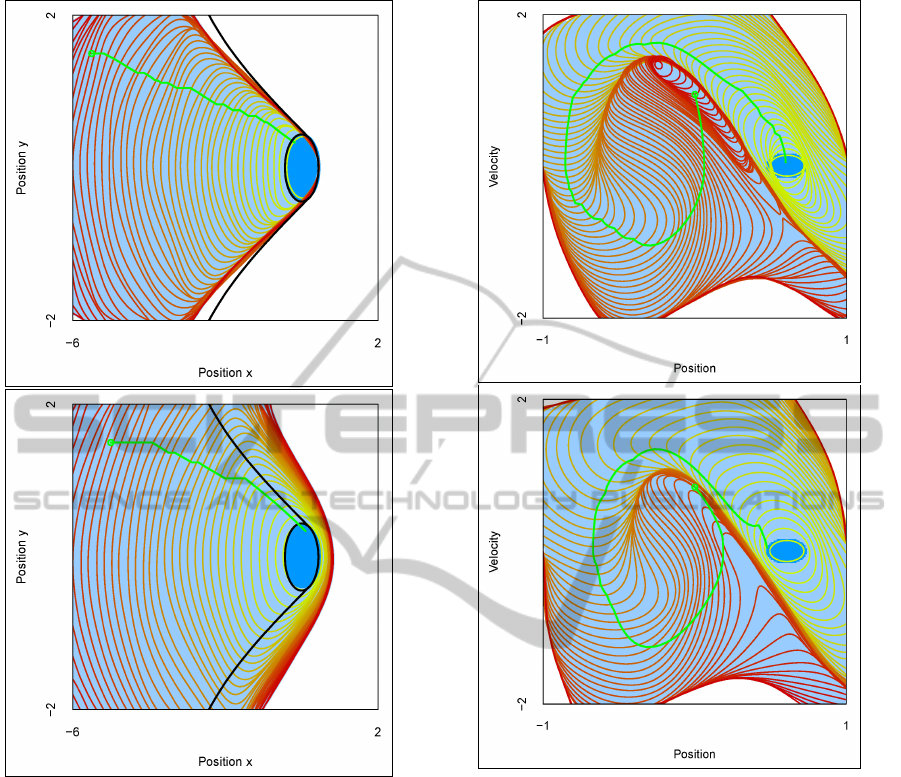
Figure 1: Approximation from inside (top) and from outside
(bottom) for Zermelo problem. The horizontal axis repre-
sents the position x and the vertical one position y. K is
the rectangle. The capture basin is represented in blue. The
black thick line limits the boundary of the actual capture
basin. The level lines represent approximation of the con-
tours of the capture basins for successive time steps. The
grid contains 41 points by dimension. The optimisation is
made on 4 time steps, with dt = 0.05. Each figure presents
an example of trajectory (in green) using the SVM optimal
controller.
5 DISCUSSION
We proposed an algorithm that approximates capture
basins and minimal time functions, using a classifi-
cation procedure, in two variants (inner and outer).
The inner approximation can be used to define a opti-
mal controller that guarantees to find a series of con-
trols that allows the system to reach the target. SVMs
Figure 2: Inner (top) and outer (bottom) approximation for
the car on the hill problem. The grid contains 51 points by
dimension. The optimisation is made on 2 time steps. An
example of an optimal trajectory is depicted in green.
appear as a particularly relevant classification proce-
dure for this approach, because they provide parsimo-
nious representations of the capture basins and en-
able to use optimization techniques to compute the
controls. This latter point is particularly important to
deal with high dimensional control space. The parci-
monious property may allow to define compact and
fast controller, even for high dimensional state space.
However, although we generally manage to find pa-
rameters in which the result respect the conditions of
convergence, this is not guaranteed. Therefore, con-
sidering other learning algorithms that would be even
more appropriate seems a relevant research direction.
A second direction of research is to investigate other
problems that could be solved by this approach. For
instance in the definition of resilience proposed by
ICINCO 2011 - 8th International Conference on Informatics in Control, Automation and Robotics
38

(Martin, 2004), there is a problem of target hitting in
which a cost function is associated with the states. We
think that our approach could easily be adapted to this
problem.
REFERENCES
Aubin, J.-P. (1991). Viability theory. Birkh
¨
auser.
Bayen, A., E., C., and & Tomlin, C. (2002). Guaranteed
overapproximations of unsafe sets for continuous and
hybrid systems: Solving the hamilton-jacobi equation
using viability techniques. Lecture Notes In Computer
Science, 2289:90–104.
Cardaliaguet, P., Quincampoix, M., and Saint-Pierre, P.
(1998). Set-Valued Numerical Analysis for Optimal
control and Differential Games. Annals of the Inter-
national Society of Dynamic Games.
Chang, C.-C. and Lin, C.-J. (2001). Libsvm: a library for
support vector machines.
Deffuant, G., Chapel, L., and Martin, S. (2007). Approxi-
mating viability kernels with support vector machines.
IEEE transactions on automatic control, 52(5):933–
937.
Frankowska, H. (1989). Optimal trajectories associated
with a solution of the contingent hamilton-jacobi
equation. Applied Mathematics and Optimization,
19(1):291–311.
Lhommeau, M., Jaulin, L., and Hardouin, L. (2007). Inner
and outer approximation of capture basin using inter-
val analysis. In 4th International Conference on Infor-
matics in Control, Automation and Robotics (ICINCO
2007).
Lygeros, J. (2004). On reachability and minimum cost op-
timal control. Automatica, 40:917–927.
Martin, S. (2004). The cost of restoration as a way of defin-
ing resilience: a viability approach applied to a model
of lake eutrophication. Ecology and Society, 9(2).
Mitchell, I., Bayen, A., and Tomlin, C. (2005). A time-
dependent Hamilton-Jacobi formulation for reachable
sets for continuous dynamic games. IEEE Transac-
tions on Automatic Control, 50(7):947–957.
Moore, A. and Atkeson, C. (1995). The parti-game algo-
rithm for variable resolution reinforcement learning
in multidimensional state-spaces. Machine Learning,
21:199–233.
Saint-Pierre, P. (1994). Approximation of the viability ker-
nel. Applied Mathematics & Optimization, 29(2):187–
209.
Saint-Pierre, P. (2001). Approche ensembliste des syst
`
emes
dynamiques, regards qualitatifs et quantitatifs. Mat-
apli, Soci
´
et
´
e de Math
´
ematiques appliqu
´
ees et Indus-
trielles, page 66.
Scholkopf, B. and Smola, A. (2002). Learning with Ker-
nels: Support Vector Machines, Regularization, Opti-
mization, and Beyond. MIT Press, Cambridge, MA,
USA.
Vapnik, V. (1995). The nature of statistical learning theory.
Springer Verlag.
APPENDIX
Proof of Proposition 3.1.1
Part I. First, let us prove by induction that ∀h >
0,Capt
n
⊂ C
n
h
.
By definition, Capt
0
= C = C
0
h
. Suppose that at step
n, Capt
n
⊂ C
n
h
. Consider x ∈ Capt
n+1
. Let us recall
that G(x,u) = x + ϕ(x, u).dt when x /∈ C.
Defining B
h
(x,d) the set of points of K
h
such that
|x − x
h
| ≤ d, we can easily show that condition (16)
can be rewritten as:
B
h
(x,h) ⊂ C
n
h
⇒ x ∈ C
n
h
. (27)
By definition, we know that there exists u ∈ U such
that G(x, u) ∈ Capt
n
, which implies that for all
x
h
∈ B
h
(x,h), d (G(x
h
,u),Capt
n
) ≤ µh, because G is
µ-Lipschitz.
Moreover, for all x
h
∈ B
h
(x,h), d(G(x
h
,u),C
n
h
) ≤ µh,
because, by hypothesis, Capt
n
⊂ C
n
h
. Thus x
h
∈ C
n+1
h
.
Therefore, x ∈ C
n+1
h
(because of condition (27)).
We can thus conclude Capt
n+1
⊂ C
n+1
h
.
Part II. Now, we prove by induction that for
any n, C
n
h
→ Capt
n
when h → 0.
Suppose now that for a given value n, C
n
h
→ Capt
n
when h → 0.
Because Capt
n
⊂ C
n
h
, we have:
∀x ∈ K | x /∈ Capt
n
, ∃h > 0 | x /∈ C
n
h
.
Now, consider x ∈ K such that x /∈ Capt
n+1
.
This implies that for all u ∈ U such that
d (G(x,u),Capt
n
) > 0. One can choose h
0
> 0 and h
such that for all u ∈ U, d (G(x,u),Capt
n
) > h
0
+ µλh.
Condition (15) can be rewritten as:
B
h
(x,λh) ⊂
C
n
h
⇒ x ∈ C
n
h
. (28)
In this case, for all x
h
∈ B
h
(x,λh), all u ∈ U,
d (G(x
h
,u),Capt
n
) > h
0
, because G is µ-Lipschitz.
Since C
n
h
→ Capt
n
when h → 0, there exists h, such
that, for all x
h
∈ B
h
(x,λh), and all u ∈ U, G(x
h
,u) ∈
C
n
h
, hence x
h
∈ C
n
h
. Hence, there exists h such that
x /∈ C
n
h
(because of condition 27).
Therefore C
n+1
h
→ Capt
n+1
when h → 0.
Conclusion. Capt
n
⊂ C
n
h
and C
n
h
→ Capt
n
then C
n
h
is
an outer approximation of the capture basin at time
n.dt, which tends to the actual capture basin when the
resolution of the grid h tends to 0.
INNER AND OUTER CAPTURE BASIN APPROXIMATION WITH SUPPORT VECTOR MACHINES
39

Proof of Proposition 3.1.2
Part I. We begin to show by induction that C
n
h
⊂
Capt
n
.
Suppose that C
n
h
⊂ Capt
n
and consider x ∈ C
n+1
h
.
Because of condition (20):
∃x
h
∈ C
n+1
h
such that |x − x
h
| < h.
By definition of C
n+1
h
:
∃u ∈ U such that d
a
(G(x
h
,u),C
n
h
) > µh.
By hypothesis of induction C
n
h
⊂ Capt
n
, hence
: d
a
(G(x
h
,u),Capt
n
) > µh. By hypothesis
on G, |G(x
h
,u) − G(x,u)| < µ|x
h
− x|, hence
d
a
(G(x,u),Capt
n
) > 0. Therefore x ∈ Capt
n+1
. Thus
C
n+1
h
⊂ Capt
n+1
.
Part II. We prove by induction that, when h → 0,
C
n
h
→ Capt
n
.
Suppose that C
n
h
→ Capt
n
when h → 0.
Because C
n
h
⊂ Capt
n
, we have:
∀x ∈ Capt
n
| d
a
(x,∂Capt
n
) > 0,∃h > 0 | x ∈ C
n
h
.
We use the rewriting of condition (21):
B
h
(x,λh) ∩C
n
h
⇒ x ∈ C
n
h
. (29)
Consider x ∈ Capt
n+1
such that d
a
(x,∂Capt
n+1
) > 0
. One can choose h such that d
a
(x,∂Capt
n+1
) >
(µ + λ)h. With such a choice, for each x
h
∈ B
h
(x,λh),
d
a
(x
h
,∂Capt
n+1
) > µh, hence, there exists u ∈ U
such that d
a
(G(x
h
,u),Capt
n
)) > 0 (because G is µ-
Lipschitz).
By induction hypothesis, there exists h such that
d
a
G(x
h
,u),C
n
h
> µh, hence x
h
∈ C
n+1
h
. Taking the
smallest value of h this is true for all x
h
∈ B
h
(x,λh).
Therefore x ∈ C
n+1
h
(because of condition (29)).
Therefore C
n+1
h
→ Capt
n+1
when h → 0.
Conclusion. C
n
h
⊂ Capt
n
and C
n
h
→ Capt
n
then C
n
h
is an inner approximation of the capture basin in fi-
nite time n.dt, which tends to the actual capture basin
when the resolution of the grid tends to 0.
ICINCO 2011 - 8th International Conference on Informatics in Control, Automation and Robotics
40
