
FORCASTING OF RENEWABLE ENERGY LOAD WITH
RADIAL BASIS FUNCTION (RBF) NEURAL NETWORKS
Otilia Elena Dragomir
Automation, Computer Science and Electrical Engineering Department, Electrical Engineering Faculty
Valahia University of Targoviste, 18 Unirii Av., Targoviste, Romania
Florin Dragomir
Automation, Computer Science and Electrical Engineering Department, Electrical Engineering Faculty
Valahia University of Targoviste, 18 Unirii Av., Targoviste, Romania
Eugenia Minca
Automation, Computer Science and Electrical Engineering Department, Electrical Engineering Faculty
Valahia University of Targoviste, 18 Unirii Av., Targoviste, Romania
Keywords: RBF, Neural networks, Load renewable energy, Forecasting.
Abstract: This paper focus on radial- basis function (RBF) neural networks, the most popular and widely-used
paradigms in many applications, including renewable energy forecasting. It provides an analysis of short
term load forecasting STLF performances of RBF neural networks. Precisely, the goal is to forecast the
DPcg (difference between the electricity produced from renewable energy sources and consumed), for
short- term horizon. The forecasting accuracy and precision, in capturing nonlinear interdependencies
between the load and solar radiation of these neural networks are illustrated and discussed using a data
based obtain from an experimental photovoltaic amphitheatre of minimum dimension 0.4kV/10kW.
1 INTRODUCTION
Research efforts on artificial neural networks
(ANNs) for forecasting are considerable. The
literature is vast and growing. In the forecasting
works, the term “forecasting” is called also
prediction or prognosis. This reveals that there is no
consensual acceptation of term. Due to these facts,
in this article the forecasting will be associated with
the notion of prediction and will determine the
future state of the analyzed system the closest
possible to the future real state of the system (O.
Dragomir. 2010).
Different forecasting time horizons are employed
in prediction approaches (day-ahead, hour-ahead) in
relation with the application. Short term load
forecasting (STLF) samples the information on an
hourly (or half hourly) basis, or even a daily basis
(for load peak prediction) so is defined as varying
from a few minutes up to a few weeks ahead. This
type of forecasting is important because the national
grid requires DPcg (difference between the
electricity produced and consumed) values at any
moment in the day. Traditionally, hourly forecasts
with a lead time between one hour and seven days
are required for the scheduling and control of power
systems. From the perspective of the system
operators and regulatory agencies, STLF is a source
of primary information for safe and reliable
operation of the system. For producers also, this type
of forecasting is a basic tool for determining the
optimal utilization of generators and power stations,
as some facilities are more efficient than others.
In this context, this paper provides architecture
of RBF, capable to forecast the DPcg for short- term
horizon. The proposed structures are applied on a
data based obtain from an experimental photovoltaic
amphitheatre of minimum dimension (0.4kV/10kW),
located in the east-centre region of Romania, more
precisely in the city of Targoviste (ICOP- DEMO.
409
Elena Dragomir O., Dragomir F. and Minca E..
FORCASTING OF RENEWABLE ENERGY LOAD WITH RADIAL BASIS FUNCTION (RBF) NEURAL NETWORKS.
DOI: 10.5220/0003534204090412
In Proceedings of the 8th International Conference on Informatics in Control, Automation and Robotics (ICINCO-2011), pages 409-412
ISBN: 978-989-8425-75-1
Copyright
c
2011 SCITEPRESS (Science and Technology Publications, Lda.)

1998). The paper is organized as follows: first, it
provides an overview of RBF neural networks,
which are the most popular and widely-used
paradigms in many applications, including energy
forecasting. Second, a particular RBF architecture is
proposed to forecast the DPcg. The forecasting
accuracy and precision in capturing nonlinear
interdependencies between the load and solar
radiation of these one are illustrated and discussed.
2 RBF NEURAL NETWORKS
Actually, the systems are very complexes and the
conditioning parameters that influence system
functioning are significant. In these cases it is very
difficult to determine any sort of model for
forecasting purposes. The advantages and the
drawbacks of ANNs, leaded us to RBF neural
networks as reference tools for our approach of short
term energy balance forecasting.
The RBF network is commonly used for the
purpose of modeling uncertain and nonlinear
functions. Utilizing RBF networks or modeling
purposes could be seen as an approximation problem
in a high-dimensional space (Zemouri. 2002). A key
feature of RBF is that the output layer is nerely a
linear combination of the hidden layer signals, there
being only one hidden layer.Therefore, RBF
networks allow for a much simpler weight updating
procedure and subsequently open up greater
possibilities for stability proofs and network
robustness in that the network can be described
readily by a set of nonlinear equations
In RBF networks, determination of the number of
neurons in the hidden layer is very important
because it affects the network complexity and the
generalizing capability of the network. If the number
of the neurons in the hidden layer is insufficient, the
RBF network cannot learn the data adequately; on
the other hand, if the neuron number is too high,
poor generalization or an over learning situation may
occur (Liu, 2004). The position of the centers in the
hidden layer also affects the network performance
considerably (Simon. 2002), so determination of the
optimal locations of centers is an important task. In
the hidden layer, each neuron has an activation
function. The gaussian function, which has a spread
parameter that controls the behavior of the function,
is the most preferred activation function. The
training procedure of RBF networks also includes
the optimization of spread parameters of each
neuron. (Martinez. 2008) studied the best
approximation of Gaussian RBF neural networks
with nodes uniformly spaced. Afterwards, the
weights between the hidden layer and the output
layer must be selected appropriately. Finally, the
bias values which are added with each output are
determined in the RBF network training procedure.
In the literature, various algorithms are proposed for
training RBF networks, such as the gradient descent
(GD) algorithm (Karayiannis, 1999) and Kalman
filtering (KF) (Simon. 2002). (Ferrari. 2009) studied
the multiscale approximation problem with
hierarchical RBF neural networks. But these above
RBF methods have the same defects of the
backpropagation algorithm. They are either
instability or complicate and slow. They have
proved that the connection weight of RBF neural
networks can be obtained through various learning
algorithms; therefore the weight has certain
instability.
3 PERFORMING STLF WITH
RBF
The forecasting performances of RBF neural
networks in load forecasting, are illustrated using a
dataset with 240 data points {y(t), u(t)}, representing
the radiation [W/m2] (mean value=0.9255 and
standard deviation= 97.6705) and the DPcg [kW]
(mean value=0.8156 and standard deviation=
130.9313) , obtained from a Solar Amphitheatre
(ICOP-DEMO. 1998) and (F. Dragomir et al. 2010).
The data used are normalized before starting the
training session and de-normalized at the end of the
training.
RBF neural network, used for performing STLF,
has an input layer, one hidden layer and an output
layer. The neurons in the hidden layer contain
Gaussian transfer functions, whose outputs are
inversely proportional to the distance from the center
of the neuron (see Table 1).
Table 1: RBF parameters.
Architecture RBF
Number inputs 1
Number layers 1 hidden layer with 5 radbas neurons
1 output layer with with purelin neurons
Transfer functions gaussian - hidden layer
purelin- output layer
Performance
functions
MSE (Mean Squared Error)
MAE (Mean Absolute Error)
Initial MSE goal 0.0098
Initial spread 0.02719
For the dataset, simulations are repeated 8 times.
ICINCO 2011 - 8th International Conference on Informatics in Control, Automation and Robotics
410
Dataset is divided into train and test subsets. 60% of
the data set is selected as the training data and
remained data set is selected as the testing data. For
each run, the number of neurons, deviations of the
radial units, MAE (Mean Absolute Error) and MSE
(Mean Square Error) are computed in order to reach
the MSE goal 0.0115. The measurements based on
MSE are suggestive, because it penalizes the huge
forecasting errors. The MAE is considered that
would be an adequate error measure if the loss
function were linear (and linear in percentage, not in
absolute error); however, recent studies and the
experience of system operators indicates that the loss
function in the load forecasting problem is clearly
nonlinear, and that large errors may have disastrous
consequences for a utility.
The goal of the tests is, given training and test
data, to choose the input parameters MSE goal,
spread and Hmax (hidden layer neurons number) to
minimize MSE value.
The input parameters have been initialized with:
MSE goal= 0.0098, the minimum distance between
clusters of different classes MNDST =0.8156,
spread0 = 0.2719 and Hmax0 = 60.
In training phase the following steps are repeated
until the network's mean squared error falls below
goal or the maximum number of neurons are
reached: 1) the network is simulated, 2) the input
vector with the greatest error is found 3) a radbas
neuron is added with weights equal to that vector
and 4) the purelin layer weights are redesigned to
minimize error.
Table 2: Train and test results of RBF simulations.
Train
Test
Spread
H MSE
(*10-3)
MAE
(*10-1)
MSE
(*10-1)
0.027 25 7.4966 4.9542 6.4668
0.127 15 7.8996 1.9653 1.4197
0.227 11 9.6653 0.6805 0.1354
0.327 8 6.4121 0.5751 0.0766
0.427 7 9.3638 0.5456 0.0786
0.527 7 8.6819 0.8884 0.1448
0.627 6 8.8989 0.5706 0.0730
0.727 7 6.1955 0.9046 0.1332
The general characteristics of the RBF training
are illustrated in Table 2.
Firstly, it was investigated how the spread of the
hidden layer base function affects the network’s
performance (see Figure 1). The initial downward
trend of MSE due to spread growth isn’t the same all
over training set. This indicates the need for
consideration of a second parameter in the
evaluation of RBF training performance. This is the
number of neurons in the hidden layer.
Figure 1: MSE in relation with spread for training phase.
The number of neurons in the hidden layer is
very important in design issue of an RBF network.
Therefore, the experiments have been conducted on
different RBF networks which has 6 neurons to 25
neurons located in the hidden layer. Using more
neurons than that is needed causes an over learned
network and moreover, increases the complexity of
the RBF network (see Table 2).
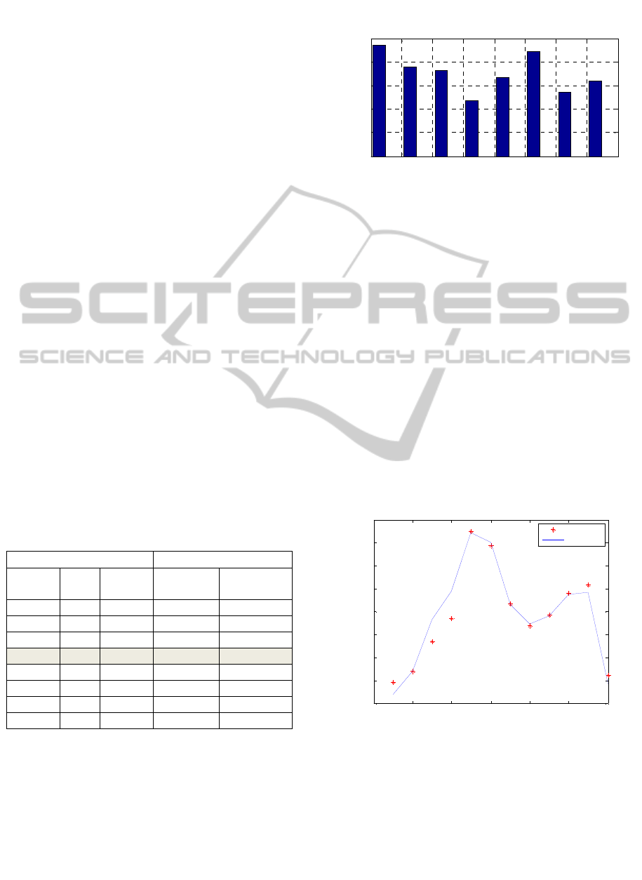
The predictions made by RBF neural network
over the test dataset in relation with the measured
outputs (targets) are illustrated in Figure 3. The
small number of test data has a bad influence over
the forecasting accuracy (see Figure 2). The output
of the RBF network is a measure of distance from a
decision hyper plane, rather than a probabilistic
confidence level The quality of the possible
solutions are calculated using MSE and MAE.
Figure 2: RBF outputs vs. targets in testing phase.
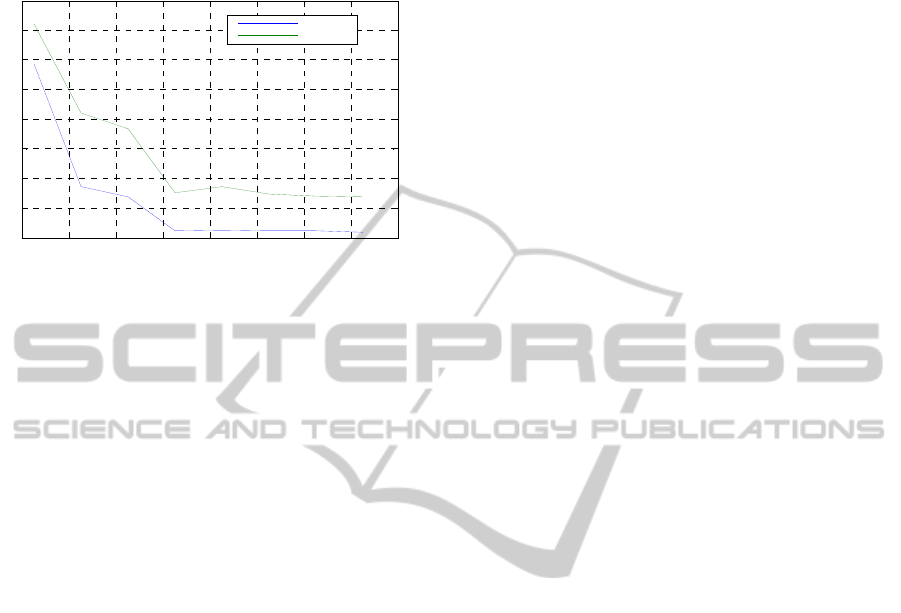
Figure 3 indicates the RBF testing errors with the
help of MAE and MSE. The Figure 3 shows that, the
growth of spread values until 0.3 has a big influence
over MAE and MSE values. These ones decreas a
lot, from 4.9542 to 0.5751 MAE and from 6.4668 to
0.0766 MSE. The trend change when the spread
reach 0.327 value. The error values increase and
0 0.1 0.2 0.3 0.4 0.5 0.6 0.7 0.8
0
0.002
0.004
0.006
0.008
0.01
spread
MSE
RBF training
0 2 4 6 8 10 12
-1.2
-1
-0.8
-0.6
-0.4
-0.2
0
0.2
0.4
RBF prediction (testing phase)
input
output
real output
RBF output
FORCASTING OF RENEWABLE ENERGY LOAD WITH RADIAL BASIS FUNCTION (RBF) NEURAL NETWORKS
411
indicate that the optimal values for spread and
number of neurons in hidden layer has to be locate.
Figure 3: MAE and MSE values of RBF in testing phase.
At the beginning, Hmax was equal with the
number of training points. The training tests with
variable number of neurons in hidden layer have
showed that 8 is the optimum number for the
neurons in hidden layer, much less than the number
of training points. At the end of RBF training, the
optimum spread value found is 0.327.
4 CONCLUSIONS AND WORK IN
PROGRESS
This paper focus on a particular neural network, the
radial basis function neural network. Considering a
data based obtain from an experimental photovoltaic
amphitheatre and MSE and MAE metrics for
forecasting performance evaluation , the simulations
and tests made in this article, put in evidence the
accuracy and precision of the particular proposed
RBF structure in capturing nonlinear
interdependencies between inputs and outputs. Due
to its good capabilities to forecast the DPcg in
relation with solar radiation, this architecture in well
suited in STLF energy applications.
The work is still in progress and the developments
are at present extended to: training the radial layer
(the hidden layer) of RBF using the Kohonen and
LVQ training algorithms, which are alternative
methods of assigning centres to reflect the spread of
data, training the output layer (whether linear or
otherwise) using any of the iterative dot product
algorithms and improving the interpretability of the
obtained predictive system.
REFERENCES
European Research Programm ICOP-DEMO 4080/98,
“Building Integration of Solar Technology”
(http://dcem.valahia.ro)
J. I. M. Martínez (2008), Best approximation of Gaussian
neural networks with nodes uniformly spaced, IEEE
Trans. Neural Netw., Vol. 19(2), pp.284–298.
Karayiannis N. B. (1999), Reformulated radial basis
neural networks trained by gradient descent,. IEEE
Trans. Neural Netw. Vol.3, pp.2230–2235.
R. Zemouri, D. Racoceanu and N. Zerhouni (2002),
Réseaux de neurones récurrents à fonctions de base
radiales: RRFR. Application au pronostic, RSTI- RIA.
Vol.16(3), pp. 307-338.
S. Ferrari, M. Maggioni & N. A. Borghese (2004),
Multiscale approximation with hierarchical radial
basis functions networks, IEEE Trans.Neural Netw.,
Vol. 15(1), pp. 178–188.
Simon D.(2002), Training radial basis neural networks
with the extended Kalman filter, Neurocomputing,
Vol. 48, pp. 455–475.
The 18th IEEE Mediterranean Conference on Control and
Automation, Marrakech, Morocco (2010), Adaptive
Neuro Fuzzy Forecasting of Renewable Energy
Balance on Medium Term, Dragomir O., Dragomir F.
& Minca E.
The 25th European Photovoltaic Solar Energy Conference
and Exhibition (25th EU PVSEC) and 5th World
Conference on Photovoltaic Energy Conversion
(WCPEC-5, Valencia, Spain (2010) Control Solution
Based on Fuzzy Logic for Low Voltage Electrical
Networks with Distributed Power from Renewable
Resources, Dragomir F., Dragomir O.. Olariu N and
Minca E.
Y. Liu; Q. Zheng; Z. Shi & J. Chen (2004), Training radial
basis function networks with particle swarms,
Comput. Sci., Vol. 3173, pp. 317–322.
0 0.1 0.2 0.3 0.4 0.5 0.6 0.7 0.8
0
0.05
0.1
0.15
0.2
0.25
0.3
0.35
0.4
spread
error
MAE and MSE for RBF testing phase
MSE
MAE
ICINCO 2011 - 8th International Conference on Informatics in Control, Automation and Robotics
412
