TRAJECTORY TRACKING CONTROL OF MOBILE
MANIPULATORS BASED ON KINEMATICS
Razvan Solea and Daniela Cernega
Departament of Automation and Electrical Engineering, “Dunarea de Jos“ University of Galati
Domneasca Street, No.47, 800008 Galati, Romania
Keywords:
Mobile manipulators, Nonlinear control, Kinematics.
Abstract:
This paper focuses on the motion planning problem of mobile manipulator systems, i.e. manipulators attached
on mobile platforms. The paper presents a methodology for generating trajectories for both the mobile plat-
form and the manipulator that will take a system from an initial configuration to a pre-specified final one,
without violating the nonholonomic constraint. The contributions of this paper come from the development
and evaluation of sliding-mode control scheme for the composite wheeled robot that facilitate maintenance of
all kinematic constraints within such systems. Given an arbitrary trajectory,the mobile-manipulator controller
must generate a smooth desired trajectory for mobile platform.
1 INTRODUCTION
Mobile Manipulator systems are typically composed
of a mobile base platform with one (or more) mounted
manipulators. Taking advantage of the increased mo-
bility and workspace provided by the mobile base,
such systems have found applications in industry
and in research principally due to their engineering
simplicity (easy to build and to control than legged
robots) and their low specific resistance (high energy
efficiency). Moving mobile manipulators systems,
present many unique problems that are due to the cou-
pling of holonomic manipulators with nonholonomic
bases.
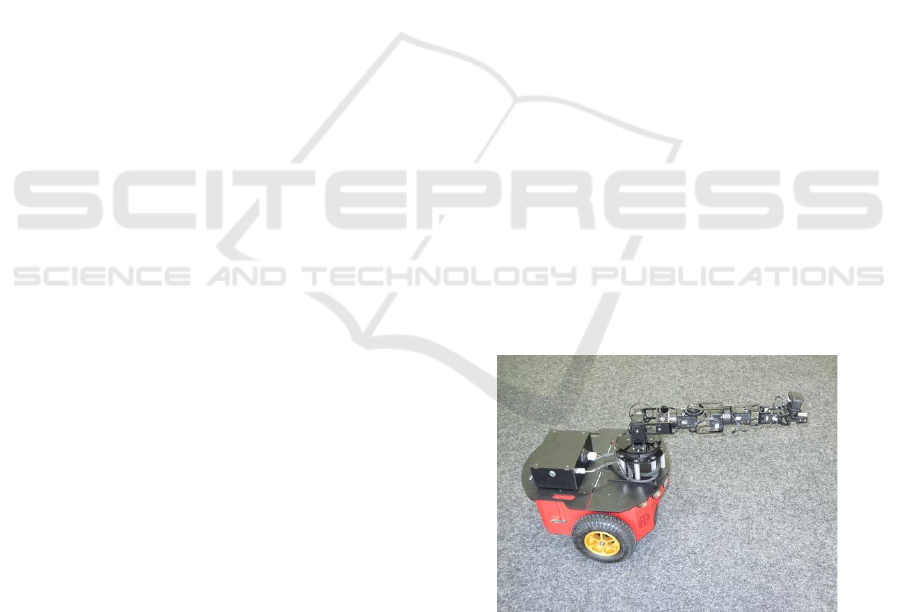
Any system combining a wheeled mobile platform
and one or several manipulators (classically arms) is
named wheeled mobile manipulators(WMM) - like in
Fig. 1. From the set of constraints and characteristics,
different approaches have been developed to control
WMM. A first class of approach is inherited from the
control schemes that have been developed for manip-
ulators. Those control schemes have been extended
to WMM in order to account for their specificities.
Among those approaches, the pioneering work of H.
Seraji1 (Seraji, 1993) can be distinguished. He pro-
posed an extension of kinematic based control laws
to the case of a mobile manipulator equipped with a
wheeled platform (unicycle) and a manipulator.
A variety of theoretical and applied control prob-
Figure 1: Pioneer 3DX mobile robot with manipular.
lems have been studied for various classes of non-
holonomic control systems. Motion planning prob-
lems are concerned with obtaining open loop controls
that steer the system from an initial state to a final
state without violating the nonholonomic constraints.
The determination of the actuator rates for a given
end effector motion of a redundant manipulator is typ-
ically an under-constrained problem. A number of
schemes have been proposed in the literature for the
resolution of the redundancy. The principal underly-
ing theme is one of optimizing some measure of per-
formance based on kinematics of the system and in
some cases extended to include the dynamics. How-
ever, in this paper, we focus our attention purely on
kinematic redundancy resolution schemes.
21
Solea R. and Cernega D..
TRAJECTORY TRACKING CONTROL OF MOBILE MANIPULATORS BASED ON KINEMATICS.
DOI: 10.5220/0003533200210027
In Proceedings of the 8th International Conference on Informatics in Control, Automation and Robotics (ICINCO-2011), pages 21-27
ISBN: 978-989-8425-75-1
Copyright
c
 2011 SCITEPRESS (Science and Technology Publications, Lda.)

The control algorithms and strategies have been
categorized into three groups, namely continuous
time-variant, discontinuous and hybrid control strate-
gies (Kolmanovsky and McClamroch, 1995), (Tanner
et al., 2003), (Sharma1 et al., 2010), (Murray, 2007),
(Klancar et al., 2009), (Mazo et al., 2004), (Zavlanos
and Pappas, 2008). Output tracking laws are easier
to design and implement, and can be embedded in a
sensorbased control architecture when the task is not
fully known in advance. For this reason, with the ex-
ception of (Fruchard et al., 2005) that takes a some-
how intermediate approach, most works on WMMs
focus on kinematic control, e.g., (Bayle et al., 2002),
(Luca et al., 2010), (Tang et al., 2008).
The rest of the paper is organized as follows: Sec-
tion 2 develops the notation and the kinematic model
for the WMM under consideration. Section 3 fo-
cuses on creation of a kinematic control law based
on sliding-mode strategy. Section 4 presents simula-
tion results to show the effectiveness of the trajectory-
traking control scheme. Section 5 concludes the paper
with a brief discussion and summarizes the avenues
for future work.
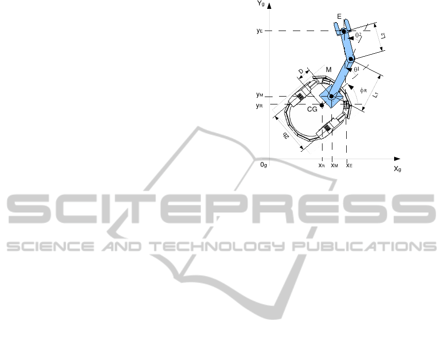
2 KINEMATIC MODEL
In this section, we present the notation and the kine-
matic model of the system under consideration. Re-
ferring to Figure 2, the WMM under consideration
consists of a differentially driven WMR base with a
mounted planar two-link manipulator (is considered
for simplity). The wheels are located at a distance of
b from the center of the wheel axle. The wheel has a
radius of r. The base of the manipulator is located at
a distance of a D from the center of the wheel axle.
The length of the first and second links are L
1
and L
2
respectively.
Motion planning has been treated mostly as a
kinematic problem where the dynamics of the system
have been generally neglected. However, with non-
holonomic systems, ignoring the dynamics reduces
the significance of the results to low speeds although
it is well documented that avoidance of obstacles,
parking maneuverability, and more motion control is
feasible at higher speeds as well.
The configuration of a WMM can be completely
described by the following generalized coordinates:
q
T
= [x
R
,y
R
,φ
R
,θ
1
,θ
2
] (1)
where [x
R
,y
R
,φ
R
] describes the configuration of the
WMR and [θ
1
,θ
2
] describes the configuration of the
planar manipulator. (x
R
,y
R
) is the Cartesian posi-
tion of the center of the axle of the WMR, φ
R
is
Figure 2: Schematic of the WMM.
the orientation of the WMR, and θ
2
, θ
2
are the rela-
tive angles that parameterize the first and second link
of the mounted manipulator. The kinematics of the
differentially-driven WMR can be represented by its
equivalent unicycle model, and described as:
˙x
R
= v
R
· cos(φ
R
)
˙y
R
= v
R
· sin(φ
R
)
˙
φ
R
= ω
R
(2)
where v
R
and ω
R
are the forward and angular veloci-
ties inputs.
The position and orientation of the end-effector in
the world frame can be derived from homogeneous
transform according to the position and orientation of
the mobile robot in the world frame, that of the end-
effector in the manipulators base frame, and the trans-
form between the mobile robot frame and the manip-
ulators base frame. The kinematics of the mobile ma-
nipulator can be described like:
x
E
= x
M
+ L
1
· cos(φ
R
+ θ
1
) + L
2
· cos(φ
R
+ θ
1
+ θ
2
)
y
E
= y
M
+ L
1
· sin(φ
R
+ θ
1
) + L
2
· sin(φ
R
+ θ
1
+ θ
2
)
(3)
where (x
M
,y
M
) is the position of mounting point M
of the mobile platform and φ
R
is the platform orienta-
tion. Eqs.3 show that the position of the end-effector
E depends on the position and the orientation of the
mobile platform. This illustrates the fact that mobile
manipulators, in contrast to fixed ones, can have an
infinite workspace.
x
M
= x
R
+ D· cos(φ
R
)
y
M
= y
R
+ D· sin(φ
R
)
(4)
By differentiating eqs. (3) and (4) will get:
ICINCO 2011 - 8th International Conference on Informatics in Control, Automation and Robotics
22

˙x
E
= v
R
· cos(φ
R
) − D· ω
R
· sin(φ
R
)−
−L
1
· (ω
R
+ ω
1
) · sin(φ
R
+ θ
1
)
−L
2
· (ω
R
+ ω
1
+ ω
2
) · sin(φ
R
+ θ
1
+ θ
2
)
˙y
E
= v
R
· sin(φ
R
) + D· ω
R
· cos(φ
R
)+
+L
1
· (ω
R
+ ω
1
) · cos(φ
R
+ θ
1
)
−L
2
· (ω
R
+ ω
1
+ ω
2
) · cos(φ
R
+ θ
1
+ θ
2
)
(5)
If the next inequality is not satisfied, then the tar-
get is outside the manipulator reach and thus the mo-
bile platform must move in order to bring the target
into the manipulator’s workspace.
|cos(φ
R
)| 6 1 ⇒
⇒ (x
E
− x
M
)
2
+ (y
E
− y
M
)
2
6 (L
1
+ L
2
)
2
(6)
The first constraint accounts for the non-
holonomic behavior of the wheels. It constrains the
velocity of the WMR to be along the rolling direc-
tion of the wheels only. Velocity perpendicular to the
rolling direction must be zero as follows :
˙x
R
· sin(φ
R
) − ˙y
R
· cos(φ
R
) = 0 (7)
This constraint, written for the manipulator attach-
ment point M, becomes:
˙x
R
· sin(φ
R
) − ˙y
R
· cos(φ
R
) +
˙
φ
R
· D = 0 (8)
3 SLIDING-MODE
CONTROLLER DESIGN
A WMM system is especially useful when the manip-
ulator task is outside the manipulator reach. There-
fore, in this section we assume that this is always the
case, in other words that inequality (6) is not satisfied
for a given target.
In this chapter is developed a control routine for
the mobile robot that allows for independent con-
trol of both the task-space (end-effector) and the
configuration-space (mobile base). As mentioned be-
fore the primary task is controlling the position of the
end-effector and attached payload. The trajectory of
the mobile base consists of a time varying function of
the position of the end-effector. Once the end-effector
final position is known, there exists extra degrees-of-
freedom that need to be controlled. These consist of
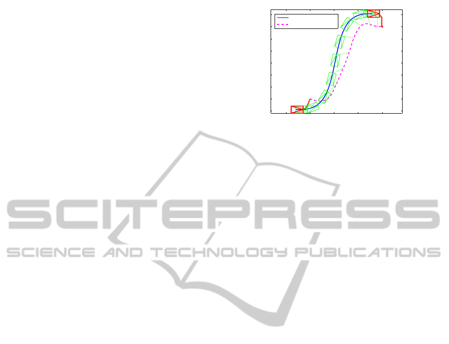
the posture of the mobile robot base and arms. This is
depicted in Figure 3, where a mobile robot is shown
moving from initial position to the final position.
Assumption: The prescribed final posture (posi-
tion, [x
E
,y
E
] and orientation [φ
R
,θ
1
,θ
2
]) is required.
Although the final position is reachable, it is virtu-
ally impossible to harvest exact orientations via con-
tinuous feedback controllers at the equilibrium point
−1 0 1 2 3
−0.5
0
0.5
1
1.5
2
2.5
3
3.5
x [m]
y [m]
Path
Path of WMM
Path of end−effector
Figure 3: Maneuver example using WMM.
of nonholonomic systems, a direct result of Brock-
etts Theorem (Brockett, 1983). Notwithstanding the
limitation, we adopt the sliding-mode technique from
(Solea and Cernega, 2009) to maneuver the WMM
into a final position such that the prescribed final ori-
entation could also be accomplished.
A trajectory planner for wheeled mobile manipu-
lators must generate smooth velocity profiles (linear
and angular) with low associated accelerations. The
trajectory planning process can be divided into two
separate parts. First, a continuous collision-free path
is generated. In a second step, called trajectory gener-
ation, a velocity profile along the path is determined.
A method to generate a velocity profile, respecting
human body comfort, for any two-dimensional path
in static environments was proposed in (Solea and
Nunes, 2007).
Uncertainties which exist in real mobile robot
applications degrade the control performance sig-
nificantly, and accordingly, need to be compen-
sated. In this section, is proposed a sliding-mode
trajectory-tracking controller, in Cartesian space,
where trajectory-trackingis achieved even in the pres-
ence of large initial pose errors and disturbances. The
application of SMC strategies in nonlinear systems
has received considerable attention in recent years.
A well-studied example of a non-holonomic system
is a WMM that is subject to the rolling without slip-
ping constraint. In trajectory tracking is an objective
to control the nonholonomic WMM to follow a de-
sired trajectory, with a given orientation relatively to
the path tangent, even when disturbances exist.
Let us define the sliding surface S = [s
1
,s
2
,s
3
,s
4
]
T
as:
s
1
= ˙x
e
+ γ
x
· x
e
s
2
= ˙y
e
+ γ
y
· y
e
+ γ
0
· sgn(y
e
) · φ
e
s
3
=
˙
θ
e1
+ γ
θ
1
· θ
e1
s
4
=
˙
θ
e2
+ γ
θ
2
· θ
e2
(9)
where γ
0
, γ
x
, γ
y
, γ
θ
1
and γ
θ
2
are positive constant pa-
rameters, x
e
, y
e
φ
e
, θ
e1
and θ
e2
are the trajectory-
tracking errors defined in Fig. 4:
TRAJECTORY TRACKING CONTROL OF MOBILE MANIPULATORS BASED ON KINEMATICS
23

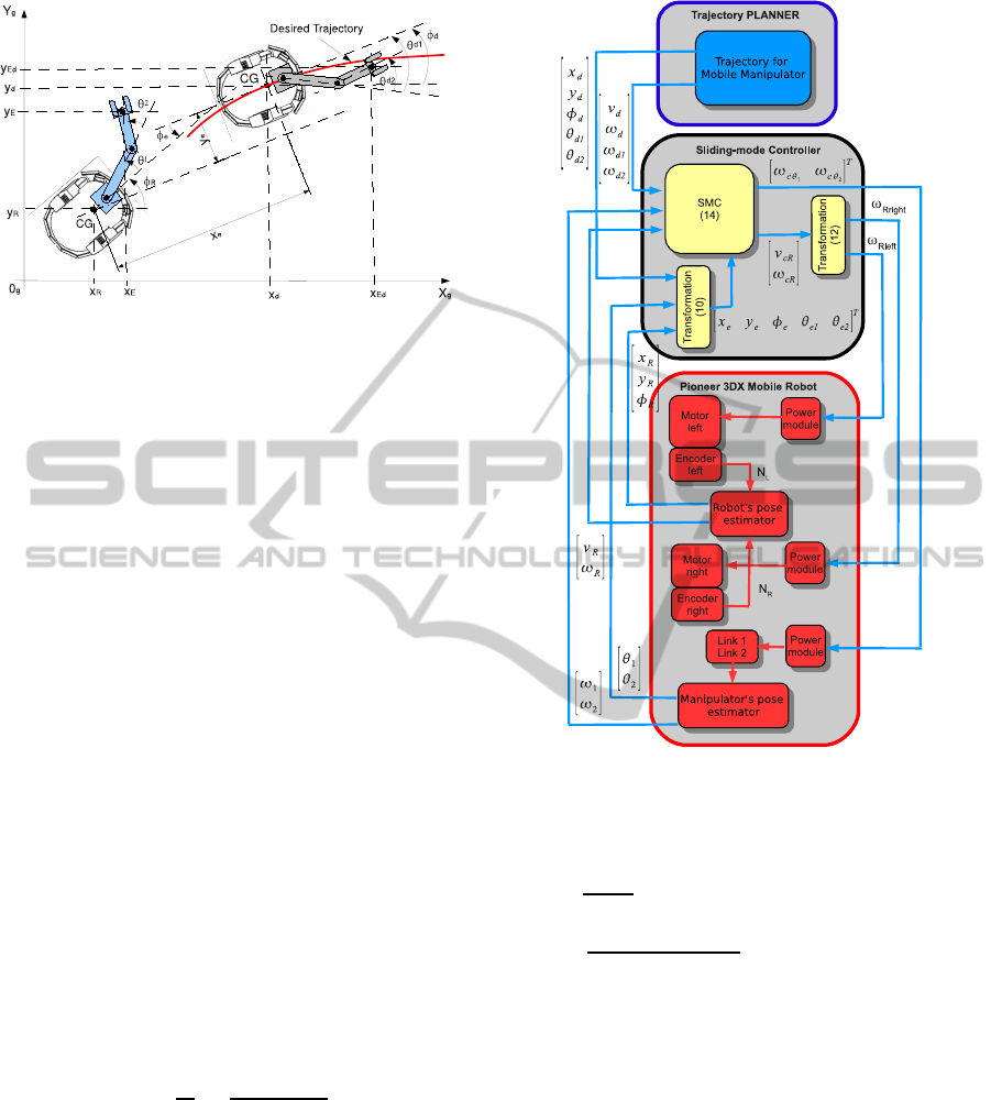
Figure 4: Lateral, longitudinal and orientation errors for
WMM.
x
e
= (x
R
− x
d
) · cos(φ
d
) + (y
R
− y
d
) · sin(φ
d
)
y
e
= −(x
R
− x
d
) · sin(φ
d
) + (y
R
− y
d
) · cos(φ
d
)
φ
e
= φ
R
− φ
d
θ
e1
= θ
1
− θ
d1
θ
e2
= θ
2
− θ
d2
(10)
If s
1
converges to zero, trivially x
e
converges to
zero. If s
2
converges to zero, in steady-state it be-
comes y
e
= γ
y
·y
e
γ
0
·sgn(y
e
)· φ
e
. For y
e
< 0 ⇒ ˙y
e
> 0
if only if γ
0
< γ
y
·|y
e
|/|φ
e
|. For y
e
> 0 ⇒ ˙y
e
< 0 if only
if γ
0
< γ
y
· |y
e
|/|φ
e
|. Finally, it can be known from s
2
that convergence of y
e
and ˙y
e
leads to convergence of
φ
e
to zero. If s
3
, s
4
converges to zero, trivially θ
e
1,
θ
e
2 converges to zero.
The reaching law is a differential equation which
specifies the dynamics of a switching function S. Gao
and Hung (Gao and J., 1993) proposed a reaching law
which directly specifies the dynamics of the switching
surface by the differential equation
˙s
i
= −p
i
· s
i
− q
i
· sgn(s
i
) (11)
where p
i
> 0, q
i
> 0, i = 1,2,3,4.
By adding the proportional rate term p
1
· s
i
, the
state is forced to approach the switching manifolds
faster when s is large. It can be shown that the reach-
ing time is finite, and is given by:
T
i
=
1
p
i
· ln
p
i
· |s
i
| + q
i
q
i
(12)
From the time derivative of (9) and using the
reaching laws defined in (11) yields:
¨x
e
+ γ
x
· ˙x
e
= −p
1
· s
1
− q
1
· sgn(s
1
)
¨y
e
+ γ
y
· ˙y
e
+ γ
0
· sgn(y
e
) ·
˙
φ
e
= −p
2
· s
2
− q
2
· sgn(s
2
)
¨
θ
e1
+ γ
θ
1
·
˙
θ
e1
= −p
3
· s
3
− q
3
· sgn(s
3
)
¨
θ
e2
+ γ
θ
2
·
˙
θ
e2
= −p
4
· s
4
− q
4
· sgn(s
4
)
(13)
From (2), (5) (10) and (13), and after some math-
ematical manipulation, we get the output commands
Figure 5: Sliding-mode trajectory tracking control architec-
ture for WMM.
of the sliding-mode trajectory-tracking controller:
˙v
cR
=
1
cos(φ
e
)
· (−p
1
· s
1
− q
1
· sgn(s
1
) − γ
x
· ˙x
e
−
−y
e
·
˙
ω
d
− ˙y
e
· ω
d
+ v
R
·
˙
φ
e
· sin(φ
e
) + ˙v
d
)
ω
cR
=
1
v
R
·cos(φ
e
)+γ
0
·sgn(y
e
)
· (−p
2
· s
2
− q
2
· sgn(s
2
)−
−γ
y
· ˙y
e
− ˙v
r
· sin(φ
e
) + x
e
·
˙
ω
d
+ ˙x
e
· ω
d
) + ω
d
˙
ω
cθ
1
= −p
3
· s
3
− q
3
· sgn(s
3
) − γ
θ
1
·
˙
θ
e1
˙
ω
cθ
2
= −p
4
· s
4
− q
4
· sgn(s
4
) − γ
θ
2
·
˙
θ
e2
(14)
The signum functions in the control laws were re-
placed by saturation functions, to reduce the chatter-
ing phenomenon (Slotine and Li, 1991).
4 SIMULATIONS AND RESULTS
In this section, simulation results for the proposed
sliding-mode controllers are presented. The simula-
tion are performed in Matlab/Simulink environment
to verify behavior of the controlled system. The pa-
rameters of the WMM model were chosen to corre-
ICINCO 2011 - 8th International Conference on Informatics in Control, Automation and Robotics
24

0 1 2 3 4
−0.5
0
0.5
1
1.5
2
2.5
3
x [m]
y [m]
Path
Desired path of WMM
Real path of WMM
Path of end−effector
Figure 6: Scenario 1 - Path of mobile manipulator.
spond as closely as possible to the real experimental
robot presented in Fig. 1 in the followingmanner: D =
0.25 [m], L
1
= 0.20 [m], L
2
= 0.40 [m], b = 0.04 [m], r
= 0.04 [m]. Wheel velocity commands, are sent to the
power modules of the follower mobile robot, and en-
coder measures N
R
and N
L
are received in the robots
pose estimator for odometric computations.
ωR
right
=
v
cR
+ b· ω
cR
r
; ωR
left
=
v
cR
− b· ω
cR
r
(15)
Figure 5 shows a block diagram of the proposed
sliding-mode controller.
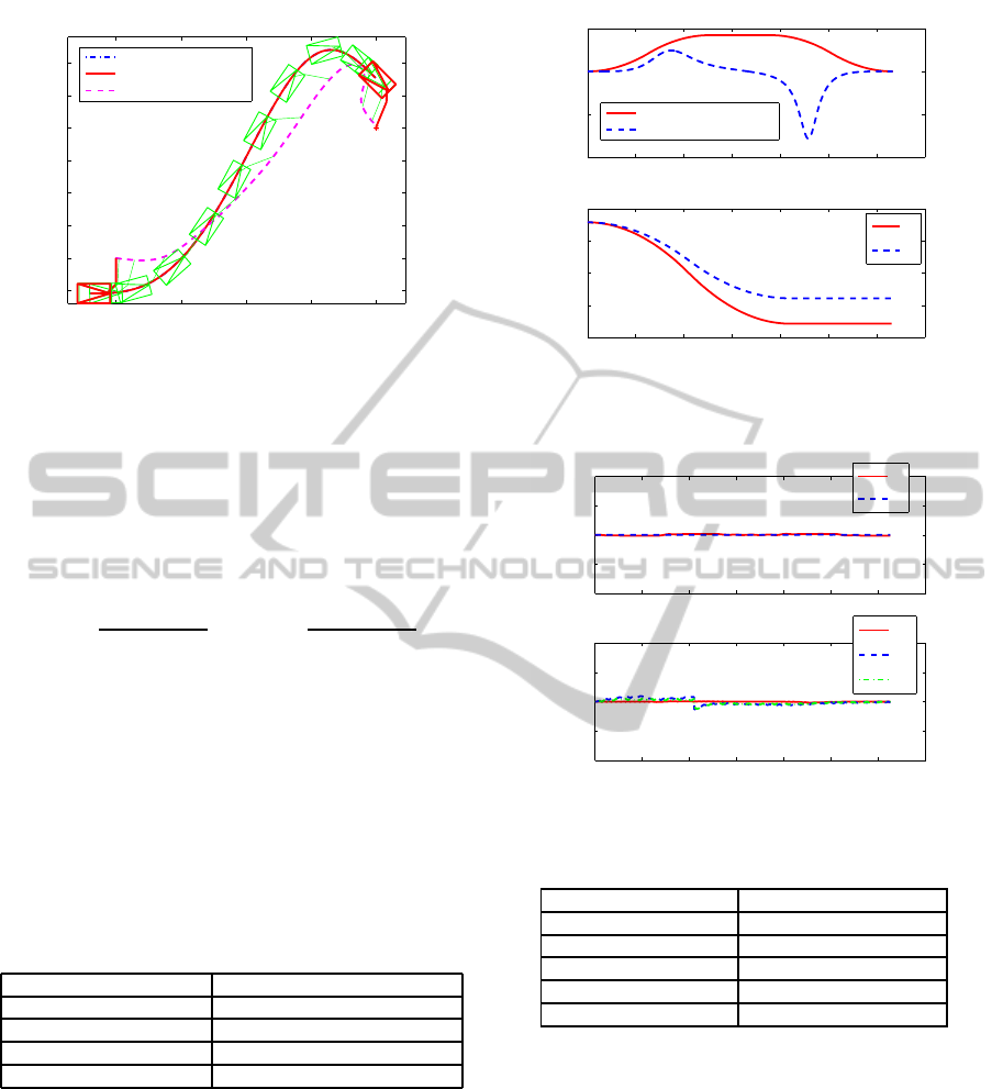
4.1 Scenario 1
The first scenario captures a situation where have to
maneuver the WMM from an initial to a final state
without pose error. The corresponding states and
workspace of the simulation are tabulated below (see
Table 1).
Table 1: Initial and final pose - Scenario 1.
Name Value
Initial position of end-effector x
E
= 0, y
E
= 0
Initial angular position φ
R
= 0, θ
1
= π/4, θ
2
= π/4
Final position of end-effector x
E
= 4, y
E
= 2
Final angular position φ
R
= −π/4, θ
1
= −π/4, θ
2
= −π/8
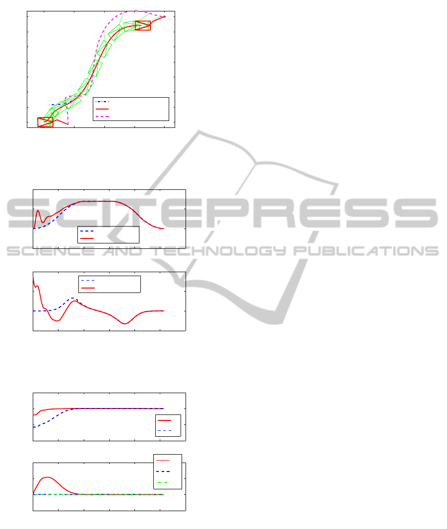
4.2 Scenario 2
The second scenario captures a situation where have
to maneuver the WMM from an initial to a final state
with initial pose error. The corresponding states and
workspace of the simulation are tabulated below (see
Table 2).
The results of the Scenario 2 are given in Figures 9
- 11. Figure 9 shows the desired and real trajectory of
the mobile platform and the real trajectory of the end-
effector. In figures 10 presents the desired and real
0 2 4 6 8 10 12 14
−2
−1
0
1
time [s]
Velocity of WMM
Linear velocity [m/s]
Angular velocity [rad/s]
0 2 4 6 8 10 12 14
−1
−0.5
0
0.5
1
time [s]
Angle of manip. [deg]
θ
1
θ
2
Figure 7: Scenario 1 - Desired velocities for WMM and the
relative angles for first and second link of the manipulator.
0 2 4 6 8 10 12 14
−0.1
−0.05
0
0.05
0.1
time [s]
x
e
and y
e
errors [m]
x
e
y
e
0 2 4 6 8 10 12 14
−10
−5
0
5
10
time [s]
Angular errors [deg]
φ
e
θ
e1
θ
e2
Figure 8: Scenario 1 - Evolution of the errors.
Table 2: Initial and final pose - Scenario 2.
Name Value
Initial pos. of end-effector x
E
= 0, y
E
= 0
Initial angular position φ
R
= 0, θ
1
= π/8, θ
2
= −π/4
Final pos. of end-effector x
E
= 3, y
E
= 3
Final angular position φ
R
= 0, θ
1
= π/4, θ
2
= −π/8
Initial pose errors of WMM x
e
= −0.20, y
e
= −0.6
velocities (linear and angular) of mobile platform. In
Fig. 11 one can observe the performances of sliding-
mode controllers. All the initial errors asymptotically
converge to zero, as shown in Fig. 11.
5 CONCLUSIONS
In this paper, we will extend the results in [18] to
multiple unanchored 2-link ma- nipulators, utilizing
again the the sliding-mode control scheme. This con-
trol scheme provides a simple but effective means of
harnessing control laws of nonlinear systems.
TRAJECTORY TRACKING CONTROL OF MOBILE MANIPULATORS BASED ON KINEMATICS
25

−1 0 1 2 3
−0.5
0
0.5
1
1.5
2
2.5
3
x [m]
y [m]
Path
Desired path of WMM
Real path of WMM
Path of end−effector
Figure 9: Scenario 2 - Path of mobile manipulator.
0 2 4 6 8 10 12
−0.5
0
0.5
1
time [s]
Linear velocity of WMM [m/s]
Desired velocity
Real velocity
0 2 4 6 8 10 12
−1
0
1
2
time [s]
Angular velocity of WMM [rad/s]
Desired velocity
Real velocity
Figure 10: Scenario 2 - Desired and real velocities for
WMM.
0 2 4 6 8 10 12
−1
−0.5
0
0.5
time [s]
x
e
and y
e
errors [m]
x
e
y
e
0 2 4 6 8 10 12
−50
0
50
100
time [s]
Angular errors [deg]
φ
e
θ
e1
θ
e2
Figure 11: Scenario 2 - Evolution of the errors.
The framework developed here lends itself well to
implementations on larger systems with further addi-
tion of mobile manipulator modules.
In future work, motivated by this work, we con-
sider the situation when multiple mobile manipulators
are grasping an object in a cooperative manner. The
purpose of controlling such coordinated system is to
control the object in the desired motion.
ACKNOWLEDGEMENTS
This work was supported by CNCSIS-UEFISCSU,
project PNII-IDEI 506/2008.
REFERENCES
Bayle, B., Fourquet, J.-Y., Lamiraux, F., and Renaud, M.
(2002). Kinematic control of wheeled mobile manip-
ulators. Proceedings of the 2002 IEEE/RSJ Interna-
tional Conference on Intelligent Robots and Systems,
1:1572–1577.
Brockett, R. W. (1983). Asymptotic stability and feedback
stabilization. In Brockett, R., Millman, R., and Suss-
mann, H. J., editors, Differential Geometric Control
Theory, pages 181–191. Birkhauser, Boston.
Fruchard, M., Morin, P., and Samson, C. (2005). A frame-
work for the control of nonholonomic mobile manip-
ulators. Rapport De Recherche INRIA, 5556:1–52.
Gao, W. and J., H. (1993). Variable structure control of non-
linear systems: A new approach. IEEE Transactions
on Industrial Electronics, 40(1):45–55.
Klancar, G., Matko, D., and Blazic, S. (2009). Wheeled
mobile robots control in a linear platoon. Journal of
Intelligent and Robotic Systems, 54(5):709–731.
Kolmanovsky, I. and McClamroch, N. (1995). Develop-
ments in nonholonomic control problems. IEEE Con-
trol Systems Magazine, 15(6):20–36.
Luca, A. D., Oriolo, G., and Giordano, P. R. (2010). Kine-
matic control of nonholonomic mobile manipulators
in the presence of steering wheels. IEEE International
Conference on Robotics and Automation, pages 1792–
1798.
Mazo, M., Speranzon, A., Johansson, K., and Hu, X.
(2004). Multi-robot tracking of a moving object using
directional sensors. IEEE International Conference on
Robotics and Automation - ICRA 2004, 2:1103–1108.
Murray, R. M. (2007). Recent research in cooperative con-
trol of multi-vehicle systems. Journal of Dynamic Sys-
tems, Measurement and Control, 129(5):571–583.
Seraji, H. (1993). An on-line approach to coordinated mo-
bility and manipulation. Proceedings of the 1993
IEEE International Conference on Robotics and Au-
tomation, 1:28–35.
Sharma1, B. N., Vanualailai, J., and Prasad, A. (2010). Tra-
jectory planning and posture control of multiple mo-
bile manipulators. International Journal of Applied
Mathematics and Computation, 2(1):11–31.
Slotine, J. and Li, W. (1991). Applied Nonliner Control.
Prentice Hall, New Jersey.
ICINCO 2011 - 8th International Conference on Informatics in Control, Automation and Robotics
26

Solea, R. and Cernega, D. (2009). Sliding mode control for
trajectory tracking problem - performance evaluation.
In ICANN (2), volume 5769 of Lecture Notes in Com-
puter Science, pages 865–874. Springer.
Solea, R. and Nunes, U. (2007). Trajectory planning
and sliding-mode control based trajectory-tracking for
cybercars. Integrated Computer-Aided Engineering,
14(1):33–47.
Tang, C. P., Miller, P. T., Krov, V. N., Ryu, J.-C., and
Agrawal, S. K. (2008). Kinematic control of a non-
holonomic wheeled mobile manipulator - a differen-
tial flatness aproach. Proceedings of ASME Dynamic
Systems and Control Conference, pages 1–8.
Tanner, H. G., Loizou, S., and Kyriakopoulos, K. J. (2003).
Nonholonomic navigation and control of cooperating
mobile manipulators. IEEE Transactions on Robotics
and Automation, 19(1):53–64.
Zavlanos, M. and Pappas, G. (2008). Dynamic assignment
in distributed motion planning with local coordina-
tion. IEEE Transaction on Robotics, 24(1):232–242.
TRAJECTORY TRACKING CONTROL OF MOBILE MANIPULATORS BASED ON KINEMATICS
27