
NONPARAMETRIC VIRTUAL SENSORS FOR SEMICONDUCTOR
MANUFACTURING
Using Information Theoretic Learning and Kernel Machines
Andrea Schirru
1
, Simone Pampuri
1,2
, Cristina De Luca
2
and Giuseppe De Nicolao
1
1
Department of Computer Science Engineering, University of Pavia, Pavia, Italy
2
Infineon Technologies Austria, Villach, Austria
Keywords:
Semiconductors, Machine learning, Entropy, Kernel methods.
Abstract:
In this paper, a novel learning methodology is presented and discussed with reference to the application of vir-
tual sensors in the semiconductor manufacturing environment. Density estimation techniques are used jointly
with Renyi’s entropy to define a loss function for the learning problem (relying on Information Theoretic
Learning concepts). Furthermore, Reproducing Kernel Hilbert Spaces (RKHS) theory is employed to handle
nonlinearities and include regularization capabilities in the model. The proposed algorithm allows to estimate
the structure of the predictive model, as well as the associated probabilistic uncertainty, in a nonparametric
fashion. The methodology is then validated using simulation studies and process data from the semiconduc-
tor manufacturing industry. The proposed approach proves to be especially effective in strongly nongaussian
environments and presents notable outlier filtering capabilities.
1 INTRODUCTION
Virtual sensors are employed in many industrial set-
tings to predict the result of an operation (most often a
measurement) when the implementation of an actual
sensor would be uneconomic or impossible (Rallo
et al., 2002). In general, a virtual sensor finds and
exploits a relation between some easily collectible
variables (input) and one or more target (output)
variables. Virtual sensor modeling techniques range
from purely physics-based approaches(Popovic et al.,
2009) to machine learning and statistical methodolo-
gies (Wang and Vachtsevanos, 2001). This paper
is motivated by a specific class of virtual sensors
used in semiconductor manufacturing, namely Vir-
tual Metrology (VM) tools. The measurement op-
erations on processed silicon wafers are particularly
time-consuming and cost-intensive: therefore, only a
small subset of the production is actually evaluated
(Weber, 2007). Conversely, Virtual Metrology tools
are able to predict metrology results at process time
for every wafer, relying only on process data: such
predictions are expected to reduce the need for ac-
tual measurement operations and, at the same time,
establish positive interactions with metrology-related
equipment tools (such as Run-to-Run controllers and
decision aiding tools).
A Virtual Metrology tool is expected to (i) find
and exploit complex, nonlinear relations between pro-
cess data and metrology results, and (ii) assess pre-
diction uncertainty in a meaningful way; in order to
achieve such goals, it is key to make the right assump-
tions on the observed data. Remarkably, a precise
characterization of the process variability is in gen-
eral hard to obtain: for instance, the observed data
might be distributed according to fat-tailed or strongly
non-Gaussian distributions, be affected by outliers or
present signs of multimodality; it is to note that such
difficulties are shared among many disciplines (Ack-
erman et al., 2010). It is intuitive that suboptimal as-
sumptions are likely to result in ineffective predictive
models. In this paper, we present a novel methodol-
ogy, inspired by Information Theoretic Learning the-
ory (Principe, 2010), to tackle such an issue employ-
ing a regularized Reproducing Kernel Hilbert Space
(RKHS) framework jointly with nonparametric den-
sity estimation techniques. The proposed approach is
able to simultaneously estimate nonlinear predictive
models and the associated prediction uncertainty, en-
abling the delivery of probabilistic predictions. The
paper is structured as follows:
• Section 2 introduces the needed elements of ma-
chine learning and Kernel methods.
349
Schirru A., Pampuri S., De Luca C. and De Nicolao G..
NONPARAMETRIC VIRTUAL SENSORS FOR SEMICONDUCTOR MANUFACTURING - Using Information Theoretic Learning and Kernel Machines.
DOI: 10.5220/0003520403490358
In Proceedings of the 8th International Conference on Informatics in Control, Automation and Robotics (ICINCO-2011), pages 349-358
ISBN: 978-989-8425-75-1
Copyright
c
2011 SCITEPRESS (Science and Technology Publications, Lda.)

• Section 3 presents and justifies the proposed ap-
proach from a theoretical point of view.
• Section 4 tests the proposed methodology against
simulation studies and data from the semiconduc-
tor manufacturing environment.
Appendix A is devoted to numerical techniques
used to solve the proposed problem, while Appendix
B contains mathematical proofs.
2 MACHINE LEARNING AND
KERNEL METHODS
The goal of a learning task is to estimate, from data, a
relationship between an input space X and an output
space Y . In order to achieve such result, it is neces-
sary to rely on a set of observations S = {x
i
∈ X ,y
i
∈
Y ,i = 1,..., N}. In other words, the goal is to find
a map f : X → Y such that, given a new observation
{x
new
∈ X ,y
new
∈ Y }, f(x
new
) will adequately pre-
dict y
new
. In this framework, S is called a training set
and the function f is an estimator. In the follow-
ing, let f depend on a set of parameters θ, such that
f(x) := f(x;θ); the optimization of θ with respect to
some suitable criterion (function of S and θ) leads to
the creation of a predictive model.
2.1 Regularized Machine Learning
In this paper, a regularized machine learning setting is
employed to introduce and test the proposed method-
ology: the estimator f is found by minimizing some
loss function J (θ) with respect to θ. Such loss func-
tion is usually the sum of a loss term L and a regular-
ization term R , so that
J (θ) = L (θ) + λR (θ) (1)
In this framework, given a model specified by θ, L
measures the quality of approximation on the train-
ing set S and R is a measure of the complexity of the
model. Intuitively, the coexistence of L and R relates
to a tradeoff between model regularity and perfor-
mances on S . The regularization parameter λ ∈ R
+
acts as a tuning knob for such tradeoff: as λ grows, the
order of the selected model gets lower and lower. In
this paradigm, a learning algorithm is entirely speci-
fied by (i) the loss term L (θ), (ii) the regularization
term R (θ) and (iii) the estimator structure f(x;θ).
Remarkably, this structure assumes that the prediction
of a generic y
i
can be obtained, at best, up to a random
uncertainty (depending on L ). In other words, adopt-
ing an additive error paradigm, it is implied that
y
i
= f(x
i
) + ε
i
where ε
i
is a random variable whose distribution
depends on L .
In the following, let X ≡ R
p
and, with no loss of
generality, Y ≡ R. The goal is to build a map f :
R
p
→ R of the relationship between an input dataset
X ∈R
N×p
and an array of target observationsY ∈R
N
.
Furthermore, let x
i
be the i-th row of X, and y
i
be the
i-th entry of Y.
2.2 Linear Predictive Models
Perhaps the most notable example of estimation tech-
nique is the method of Least Squares, that can be
traced back to Gauss and Legendre. Such method-
ology assumes a linear relationship between the input
and output spaces, so that
f(x
i
) := f(x
i
;w) = x
i
w (2)
where w is a p-variate vector of parameters. Fur-
thermore, let L be the sum of squared residuals
L (w) =
N
∑
i=1
(y
i
− f(x
i
))
2
(3)
and let R (w) ≡ 0. The optimal w
∗
(minimizer of
L (w)) is then
w
∗
= (X
′
X)
−1
X
′
Y
When a new input observation x
new
is available,
the optimal least squares prediction of y
new
is
ˆy
new
= E[y
new
|x
new
] = x
new
w
∗
Equation (3) implies a Gaussian distributed ε
i
with
ε
i
∼ N(0,σ
2
)
where σ
2
is the variance of the observation un-
certainty. Notably, ˆy
new
is independent of σ
2
: it is
necessary to tune the variance term only if a prob-
abilistic output is needed (such as prediction confi-
dence intervals). Least squares is a simple yet pow-
erful method that suffers from two main drawbacks,
namely (i) overfitting in high-dimensional spaces (p
close to N) and (ii) possible ill-conditioning of the
matrix X
′
X. In order to overcome such issues, a regu-
larization term is employed: by using (2) and (3), and
letting
R (w) =
N
∑
i=1
w
2
i
Ridge Regression is obtained. More and more sta-
ble (low sum of squared coefficients) models are se-
lected as λ grows, at the cost of worsening the per-
formances on the training set. The idea behind Ridge
ICINCO 2011 - 8th International Conference on Informatics in Control, Automation and Robotics
350

Regression is that the optimal λ allows to build a pre-
dictor that includes all and only the relevant informa-
tion. The optimal Ridge Regression coefficient vector
is
w
∗
= (X
′
X + λI)
−1
X
′
Y
Similarly to least squares, it is not necessary to
explicitly address the tuning of the error variance σ
2
unless a probabilistic output is needed.
2.3 Nonlinear Predictive Models
It is apparent that (2) defines a linear relationship be-
tween the p-variate input space and the output space.
In a wide variety of applications, however, a lin-
ear model is not complex enough to obtain the de-
sired prediction performances. An unsophisticated
approach would be to adopt an expanded basis (aug-
menting the input set X with nonlinear functions of its
columns - for instance, polynomials) to tackle such
issue. It is to note, however, that this simple ap-
proach would yield computationally intractable prob-
lems also for a relatively small values of p (Hastie
et al., 2005): nonlinearities are more efficiently han-
dled using kernel-based methodologies. In the case
of Ridge Regression, consider a symmetric positive
definite matrix K ∈ R
N×N
whose entries arise from
a suitable positive definite inner product K (kernel
function), such that
K
ij
= K (x
i
,x
j
) (4)
Furthermore, consider the model structure
f(x
i
) = K
i
c (5)
where K
i
is the i-th row of K, and the regulariza-
tion term
R (c) = c
′
Kc
In this framework, c ∈ R
N
is the coefficient vec-
tor of the so-called dual form of the learning prob-
lem, and R is the norm of f in a nonlinear Hilbert
space. The resulting model f exploits a nonlinear re-
lationship (specified by K ) between X and Y. This re-
sult arises from RKHS (Reproducing Kernel Hilbert
Spaces) theory and Riesz Representation Theorem:
the kernel function K is used to establish a rela-
tionship between the p features and the N examples.
Among the most popular kernel functions, the inho-
mogeneous polynomial kernel
K (x
i
,x
j
;d) = (x
i
x
′
j
+ 1)
d
incorporates the polynomial span of X up to the
d-th grade, and the exponential kernel
K (x
i
,x
j
;ξ) = e
−
||x
i
−x
j
||
2
ξ
2
relates to an infinite-dimensional feature space
whose bandwidth is controlled by ξ
2
. The optimal
Kernel Ridge Regression coefficient vector is
c
∗
= (K + λI)
−1
Y
and the predictor is
ˆy
new
= k
new
c
∗
with k
new
= [K (x
new
,x
1
)... K (x
new
,x
N
)]. A thor-
ough review of kernel-based methodologies is beyond
the scope of this section: the interested reader can find
more information in (Scholkopf and Smola, 2002).
2.4 Learning in Nongaussian Settings
It is to note that the methodologies reviewed in this
section rely on Gaussian assumptions: the probabilis-
tic interpretation of the loss function (3) is that y
new
can be predicted, at best, with an additive Gaussian-
distributed uncertainty with fixed variance. The rea-
sons for adopting such an assumption are both histor-
ical (linking to the concept of Least Squares estima-
tion) and methodological (Central Limit Theorem and
closed form solution), but other choices are possible.
For instance, the Huber loss function (used in robust
statistics) implies a Gaussian distribution near the ori-
gin with Laplace tails and allows to reduce the weight
of outliers in the learning process. Another notable
example is the ε-insensitive loss function, that relates
to a uniform distribution between [−ε,ε] with Laplace
tails, and is mainly used in Support Vector Machines
(SVM).
Remarkably, all the loss terms described in this
section rely on parametric assumptions: the uncer-
tainty is assumed to follow a specific (known) distri-
bution depending on a set of unknown parameters. In
a real setting, however, it is often not possible (and
sometimes not even desirable) to identify the uncer-
tainty distribution in a parametric way: in such situ-
ations, a more flexible characterization is needed to
achieve the best performances. In the next section, a
learning method that achieves such flexibility is pre-
sented using Density Estimation techniques jointly
with Entropy-related criteria.
3 REGULARIZED ENTROPY
LEARNING
In this section, an entropy-based learning technique
that makes no assumptions about the uncertainty
distribution is presented and discussed. The novel
methodology will be referred to as ”Regularized En-
tropy Learning”.
NONPARAMETRIC VIRTUAL SENSORS FOR SEMICONDUCTOR MANUFACTURING - Using Information
Theoretic Learning and Kernel Machines
351
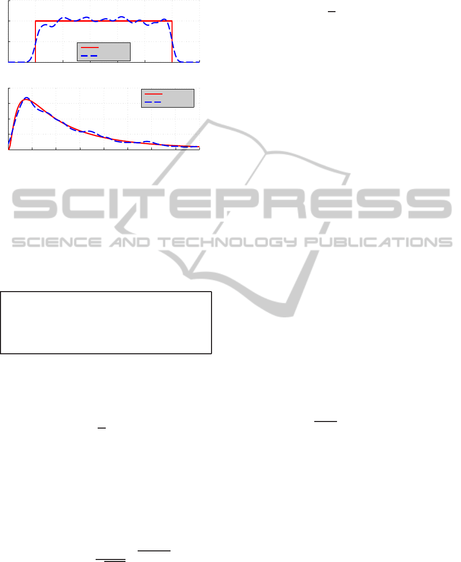
Uniform distribution
Theoretic
Estimation
Lognormal distribution
Theoretic
Estimation
Figure 1: Density estimation of uniform and lognormal dis-
tributions, using Gaussian densities.
3.1 Density Estimation and Learning
Consider a real-valued array ε = [ε
1
,. ..,ε
N
]
′
, where
every ε
i
is assumed to be independently drawn from
the same unknown distribution. In order to obtain a
nonparametric estimate of the probability density of
ε, it is convenient to resort to density estimation tech-
niques (Parzen, 1962).
Remark: it would be more correct to use the term
”kernel density estimation” (KDE). In order to
avoid confusion (the word ”kernel” has different
meaning in KDE and Kernel Methods), KDE will
be referred to as density estimation (DE).
DE techniques are able to estimate a probability
density from a set of observations, using a mixture of
predetermined distributions. Given the vector ε, the
underlying distribution is estimated as
p
ε
(x) =
1
N
N
∑
i=1
g(ε
i
;x) (6)
where g(·;x) is a nonnegative function such that
Z
+∞
−∞
g(·;x)dx = 1
It is immediate to prove that (6) is a probability
distribution. In this paper, we employ the Gaussian
density
G(µ,σ
2
;x) =
1
√
2πσ
2
e
−
(x−µ)
2
2σ
2
(7)
so that g(z;x) := G(z,σ
2
;x). Hereby σ
2
is the
bandwidth of the estimator, related to the smoothness
of the estimated density: its tuning will be discussed
in a later subsection. The density p
ε
is rewritten as
p
ε
(x) =
1
N
N
∑
i=1
G(ε
i
,σ
2
;x) (8)
that is, a Gaussian density of variance σ
2
is cen-
tered on every observation ε
i
. With reference to the
learning setting presented in the previous section, let
ε
i
be the estimation error (residual) on the i-th sample
of S , for some value of c:
ε
i
:= ε
i
(c) = y
i
−K
i
c (9)
where K
i
is the i-th row of the kernel matrix K.
In the next subsection, (8) and (9) are used to define
a loss term related to the concept of information en-
tropy.
3.2 Entropy-based Loss Term
In information theory, entropy is a measure of the un-
certainty of a random variable: while an high entropy
is associated to chaos and disorder, a quiet and pre-
dictable random variable is characterized by low en-
tropy (Gray, 2010). Notably, by minimizing the en-
tropy of a random variable, a constraint is imposed
on all its moments (Erdogmus and Principe, 2002).
For this reason, the definition of an entropy-based loss
term is desirable with respect to the Least Squares
loss term, that involves only the second moment (vari-
ance). More interesting properties of such a loss term
are investigated in (Principe et al., 2000).
Shannon’s entropy, perhaps the most notable en-
tropy measure, is defined as the expected value of the
information contained in a message. Renyi’s entropy
generalizes this concept to a family of functions de-
pending on a parameter α ≥0. Consider a continuous
random variable ε; its Renyi’s entropy H
α
(ε) is
H
α
(ε) =
1
1−α
log
Z
+∞
−∞
p
ε
(x)
α
dx (10)
We consider the quadratic Renyi’s entropy H
2
(·)
of the random variable ε|c, as
H
2
(ε(c)) = −log
Z
+∞
−∞
p
ε|c
(x)
2
dx (11)
It is easily noted that H
2
(ε) reaches its infimum
when p
ε
(x) is a Dirac Delta (complete predictability),
and its supremum when p
ε
(x) is flat over R (complete
uncertainty). In order to define the desired loss term,
we consider the following
Theorem 1. Let A ∈ R
s×s
, a ∈ R
s
, B ∈ R
t×t
, b ∈ R
t
and Q ∈R
s×t
. Let x ∈R
t
be an input variable. It holds
that
G(a,A;Qx)G(b,B;x) = G(a,A + QBQ
′
;b)G(d,D;x)
ICINCO 2011 - 8th International Conference on Informatics in Control, Automation and Robotics
352

with
D = (Q
′
A
−1
Q+ B
−1
)
−1
d = b+ DQ
′
A
−1
(a−Qb)
It is possible to express H
2
(ε) in function of a
weighted sum of Gaussian densities: this result is
summarized in the following
Proposition 1. Applying Theorem 1 (Miller, 1964)
and using (8) and (11), it holds that
H
2
(ε(c)) = −log
1
N
2
N
∑
i=1
N
∑
j=1
G(y
i
−y
j
,2σ
2
;(K
i
−K
j
)c)
!
Exploiting the symmetry of the Gaussian density,
we define
H (c) :=
2
N
2
N
∑
i=1
N
∑
j=i+1
G(y
i
−y
j
,2σ
2
;(K
i
−K
j
)c)
and observe that H (c) is equal to e
−H
2
(ε(c))
up
to an additive constant. Since the exponential trans-
formation is monotonic,
argmax
c
H (c) = argmin
c
H
2
(ε(c)) (12)
Equation (12) states that a minimum entropy es-
timator can be obtained by maximizing a mixture of
Gaussian densities with respect to the parameters vec-
tor c. In the following, since ε is entirely specified by
c, we let H
2
(c) := H
2
(ε(c)).
3.3 Regularized Entropy Learning
In this section, we consider the properties of the learn-
ing algorithm for which
L (c) = H
2
(c)
R (c) = c
′
Kc
f(y
i
) = k
i
c
The novelty of the proposed approach lies in the
RKHS regularization of an entropy-related loss term.
Consider the following
Proposition 2. Given the loss function
J (c) = H
2
(c) + λc
′
Kc (13)
it holds that
e
−J (c)
∝ H (c)G
0
N
,
K
−1
λ
;c
(14)
that is, applying an exponential transformation to
J (c), it is possible to write it as the product between
a weighted sum of Gaussian densities (H (c)) and a
Gaussian density dependent on λ.
Furthermore, it has to be considered that H
2
(c) is
shift-invariant: this result is discussed in the following
Proposition 3. Let ε(c) be a real valued vector of
residuals associated to a coefficient vector c, and let
ε(c
∗
) = ε(c) + z, where z is a real constant. It holds
that
H
2
(c) ≡ H
2
(c
∗
)
Following Proposition 3, the expected value of the
residuals represents an additional degree of freedom
to be set in advance. Without loss of generality we
choose to ensure that, given a random variable γ,
(p(γ|c) = p
ε
(x)) → (E[γ] = 0) (15)
According to Proposition 2, it is possible to write
J (c), upon a monotonic transformation, as a sum of
products of Gaussian densities. In order to define an
efficient minimization strategy for J , we consider the
following
Proposition 4. It holds that
e
−J (c)
∝
N
∑
i=1
N
∑
j=i+1
α
ij
G(d
ij
,D
ij
;c) (16)
with
α
ij
= G(y
i
,2σ
2
+
K
ii
−2K
ij
+ K
j j
λ
;y
j
)
D
ij
=
(K
i
−K
j
)
′
(K
i
−K
j
)
2σ
2
+ λK
−1
d
ij
= D
ij
(K
i
−K
j
)
′
(y
i
−y
j
)
2σ
2
where K
st
is the {s,t} entry of K, and therefore
J (c) = −log
N
∑
i=1
N
∑
j=i+1
α
ij
G(d
ij
,D
ij
;c)
!
up to an additive constant.
Proposition 4 straightforwardly applies Theorem
1 to state that it is possible to write J (c) as the loga-
rithm of a weighted sum of Gaussian densities. The
NONPARAMETRIC VIRTUAL SENSORS FOR SEMICONDUCTOR MANUFACTURING - Using Information
Theoretic Learning and Kernel Machines
353

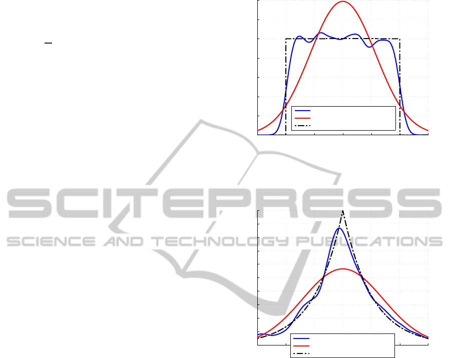
Figure 2: Graphical representation of the matrix {α
ij
} (sur-
face plot).
multiplicative coefficients α
ij
admit an interesting in-
terpretation: α
ij
, for which
0 ≤ α
ij
≤ G(0,2σ
2
;0) (17)
gets monotonically closer to its supremum as two
conditions are met: (i) y
i
is close to y
j
and (ii)
K
ii
+ K
ij
is close to 2K
ij
. Using the definition of
K
ij
= K (x
i
,x
j
), it is immediately verified that con-
dition (ii) occurs when x
i
is close to x
j
. Therefore, the
multiplicative coefficient α
ij
relates to the informa-
tion consistency between the i-th and j-th sample: in
other words, it is a measure of the similarity between
the i-th and j-th observations. This allows for two
interesting properties: (i) given a training set S , it is
possible to identify the most consistently informative
pairs of examples (Figure 2). This information can be
subsequently used, for instance, as a pruning criterion
to obtain a minimal representative dataset. Further-
more, (ii) it is possible to use {α
ij
} to discover mix-
tures in S : indeed, if it is possible to identify two sets
S
1
⊂ S and S
2
⊂ S such that, for all (i, j ∈ S
1
) and
(k,z ∈S
2
),
α
ij
≫ α
ik
α
kz
≫ α
ik
the information conveyed by S
1
and S
2
are sig-
nificantly decoupled. Figure 3 depicts a colormap of
{α
ij
} for a toy dataset with N = 30, obtained by con-
catenating two decoupled sets of observations. As ex-
pected, the upper-left and lower-right 15x15 subma-
trices show the highest values of α
ij
.
3.4 Model Estimation
In the previous subsection, we have shown that the
loss function of the proposed method is monotoni-
cally related to a weighted sum of N-variate Gaus-
sian densities. In this subsection, an optimal (entropy-
wise) regularized estimator of c is derived and em-
ployed to build a predictor for new observations. In
order to obtain c
∗
, it is necessary to solve the follow-
ing
Mixture detection with N=30
5 10 15 20 25 30
5
10
15
20
25
30
Figure 3: Mixture recognition capabilities of the coeffi-
cients α
ij
: the bright areas are self-consistent groups of ho-
mogeneous observations.
Problem 1. (Minimization of J (c)): find
c
∗
= argmin
c
e
J (c)
with
J (c) = −log
N
∑
i=1
N
∑
j=i+1
α
ij
G(d
ij
,D
ij
;c)
!
Since the exponential transformation is monotonic,
the minimizer of e
J (c)
minimizes also J (c); the expo-
nential formulation yields, however, simpler deriva-
tives. Implementation details about the solution of
Problem 1 are reported in Appendix A. The esti-
mate c
∗
represents a compromise between the RKHS
norm of f, R (c), and Renyi’s second order entropy of
the estimation errors, H
2
(c). Additionally, H
2
(c
∗
) is
the minimum reachable entropy configuration for the
dataset S for a given value of λ. As c
∗
is obtained by
solving Problem 1, it is necessary to set the additional
degree of freedom discussed in Proposition 3: the bias
term B is computed as
B := mean({ε
i
}) =
1
N
N
∑
i=1
(y
i
−K
i
c
∗
)
It is then possible to compute predictions when-
ever a new observation x
new
is available. Using the
real-valued array
k
new
= [K ( ˜x
new
,x
1
)... K ( ˜x
new
,x
N
)]
the estimator ˆy
new
is
ˆy
new
= E[y
new
|x
new
] = k
new
c
∗
(18)
ICINCO 2011 - 8th International Conference on Informatics in Control, Automation and Robotics
354
Furthermore, the prediction uncertainty γ can be es-
timated using a Leave-One-Out approach: let
p(γ) =
1
N
N
∑
i=1
G(y
i
−K
i
c
∗
(i)
−B
(i)
,σ
2
;x) (19)
where c
∗
(i)
and B
(i)
solve Problem 1 using the re-
duced dataset S
(i)
= S \{x
i
,y
i
}. The probabilistic form
of the predictor is then
y
new
= ˆy
new
+ γ (20)
where ˆy
new
is deterministic and γ is a random vari-
able.
It is to be noted that the solution of Problem 1
was obtained for fixed bandwidth σ
2
and regulariza-
tion parameter λ. In practice, however, it is generally
needed to estimate such parameters from data as well.
In the presented univariate case, the tuning of such
parameters was efficiently performed by means of a
Generalized Cross Validation (GCV) approach. It is
also possible, if there is not enough data to perform
GCV, is to tune σ
2
relying on some theoretical crite-
rion, such as Silverman’s rule (Silverman, 1986).
4 RESULTS
In this section, Regularized Entropy Learning (REL)
is tested against simulated datasets and data com-
ing from the semiconductor manufacturing industry.
In order to understand the potential of the proposed
approach, its performances are compared with Ker-
nel Ridge Regression (KRR). The performance gap
between Regularized Entropy Learning and Kernel
Ridge Regression is expected to vary: intuitively, if
the real uncertainty distribution is strongly nongaus-
sian, REL is expected to outperform KRR. For all the
experiments, RMSE was used as metric; the parame-
ters of both methods were tuned by means of GCV.
4.1 Simulated Datasets
Two datasets (100 training, 50 validation and 50 test
observations) were generated using strongly nongaus-
sian uncertainty distributions. In the first case, a uni-
form random variable was employed; in the second
case, the uncertainty was modeled as a Laplace dis-
tribution. Multiplicative (5x) outliers were inserted
(with 10% probability) in each dataset to test the
robustness of the proposed methodology. Table 1
presents the RMSE ratios for the four simulated ex-
periments: as expected, the best results are obtained
with the Laplace distribution (whose power law is
−3 −2 −1 0 1 2 3
0
0.05
0.1
0.15
0.2
0.25
0.3
0.35
p
Error distributions
Regularized Entropy Learning (p( γ))
Kernel Ridge Regression
Real Distribution
Figure 4: Error distributions for the prediction of a simu-
lated dataset with uniform uncertainty: the nonparametric
estimation of p(γ) allows the proposed methodology to out-
perform KRR.
−3 −2 −1 0 1 2 3
0
0.05
0.1
0.15
0.2
0.25
0.3
0.35
0.4
0.45
0.5
p
Error distributions
Regularized Entropy Learning (p( γ))
Kernel Ridge Regression
Real Distribution
Figure 5: Error distributions for the prediction of a simu-
lated dataset with Laplace-distributed uncertainty: the fat
tails of the Laplace distribution are correctly recognized
by REL, while the Gaussian assumptions of KRR fail to
achieve the best prediction results.
hardly approximated by a Gaussian). Figures 4 and 5
show the uncertainty distributions considered by REL
and KRR: the advantage of the proposed approach in
such situations is clear.
4.2 Semiconductor Dataset
REL was tested against a set of homogeneous obser-
vations from the semiconductor manufacturing envi-
ronment (courtesy of the Infineon Austria facility in
Villach). Specifically, a homogeneous dataset con-
sisting of 239 measured wafers was collected from a
Chemical Vapor Deposition (CVD) equipment. Ev-
ery wafer is characterized by 30 input variables and 9
thickness measurements (associated to different sites
on the wafer). Four experiments were conducted:
NONPARAMETRIC VIRTUAL SENSORS FOR SEMICONDUCTOR MANUFACTURING - Using Information
Theoretic Learning and Kernel Machines
355
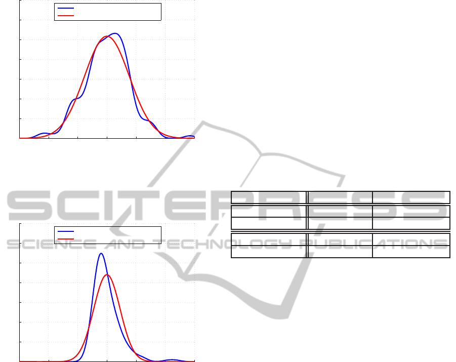
−3 −2 −1 0 1 2 3
0
0.1
0.2
0.3
0.4
0.5
0.6
0.7
Thickness average
p
Error distributions
Regularized Entropy Learning (p( γ))
Kernel Ridge Regression
Figure 6: Error distributions for the prediction of average
thickness with no outliers: notably, in this case the Gaussian
assumptions are verified, and KRR performs better than the
proposed methodology.
−3 −2 −1 0 1 2 3
0
0.2
0.4
0.6
0.8
1
1.2
1.4
Thickness std
p
Error distributions
Regularized Entropy Learning (p( γ))
Kernel Ridge Regression
Figure 7: In the prediction of standard deviation, the density
estimated distribution is skewed and strongly nongaussian
(both the distributions in this Figure has expected value 0).
Thanks to this better understanding of the uncertainty dis-
tribution, the proposed methodology performs well in this
setting.
• Predict the average layer thickness (with and
without outliers).
• Predict the standard deviation (9 points) of layer
thickness (with and without an outliers).
In order to produce outlier-free experiments, a
standard outlier elimination technique based on Ma-
halanobis distance was employed. The original
dataset was split in 3 consecutive groups: a train-
ing dataset of 150 wafers, a validation dataset of 50
wafers and a test dataset of 39 wafers. The validation
dataset was used to tune the hyperparameters, while
the algorithms were compared on the test dataset.
The results of this experiment are reported in Ta-
ble 1. Notably, the Gaussian assumptions are verified
for the average thickness without outliers (Figure 6):
in this case, KRR performs better than REL. On the
other hand, the presence of outliers in the dataset sig-
nificantly degrades the performances of KRR, while
the proposed methodology proves to be naturally ro-
bust. Perhaps the most interesting result comes from
the prediction of standard deviation: thanks to the
skewed uncertainty distribution associated to the stan-
dard deviation measurements (Figure 7), REL outper-
forms KRR.
Table 1: RMSE ratios REL/KRR: the proposed methodol-
ogy shows natural robustness with respect to outliers, and
performs better than KRR when Gaussianity assumptions
are less realistic. The best result is in bold, while the worst
result is in red.
With outliers Without outliers
Uniform 0.61 0.67
Laplace 0.52 0.56
Thickness Avg. 0.98 1.17
Thickness Std. 0.73 0.89
5 CONCLUSIONS
In this paper, a novel learning methodology is pro-
posed relying on information theory concepts in a
regularized machine learning framework. This study
is motivated by the application of Virtual Metrology
in semiconductor manufacturing. The estimation of
a nonlinear predictive model, jointly with the associ-
ated uncertainty distribution, is achievedin a nonpara-
metric way using a metric based on Renyi’s entropy
and regularized with a RKHS norm. The proposed
methodology, namely Regularized Entropy Learning
(REL), has been tested with promising results on sim-
ulated datasets and process data from the semiconduc-
tor manufacturing environment. Specifically, the pro-
posed approach presents a clear advantage in outlier-
intensive and strongly nongaussian environments: for
this reasons, REL is a strong candidate for the use in
an industrial setting, where a flexible assessment of
data variability is key to achieve good predictive per-
formances.
REFERENCES
Ackerman, F., Stanton, E., and Bueno, R. (2010). Fat tails,
exponents, extreme uncertainty: Simulating catastro-
phe in DICE. Ecological Economics, 69(8):1657–
1665.
ICINCO 2011 - 8th International Conference on Informatics in Control, Automation and Robotics
356

Carreira-Perpi˜n´an, M. (2002). Mode-finding for mixtures of
Gaussian distributions. Pattern Analysis and Machine
Intelligence, IEEE Transactions on, 22(11):1318–
1323.
Erdogmus, D. and Principe, J. (2002). An error-entropy
minimization algorithm for supervised training of
nonlinear adaptive systems. Signal Processing, IEEE
Transactions on, 50(7):1780–1786.
Gray, R. (2010). Entropy and information theory. Springer
Verlag.
Hastie, T., Tibshirani, R., Friedman, J., and Franklin, J.
(2005). The elements of statistical learning: data min-
ing, inference and prediction. The Mathematical In-
telligencer, 27(2):83–85.
Miller, K. (1964). Multidimensional gaussian distributions.
Wiley New York.
Parzen, E. (1962). On estimation of a probability density
function and mode. The annals of mathematical statis-
tics, 33(3):1065–1076.
Popovic, D., Milosavljevic, V., Zekic, A., Macgearailt, N.,
and Daniels, S. (2009). Impact of low pressure plasma
discharge on etch rate of SiO2 wafer. In APS Meeting
Abstracts, volume 1, page 8037P.
Principe, J. (2010). Information Theoretic Learning:
Renyi’s Entropy and Kernel Perspectives. Springer
Verlag.
Principe, J., Xu, D., Zhao, Q., and Fisher, J. (2000). Learn-
ing from examples with information theoretic criteria.
The Journal of VLSI Signal Processing, 26(1):61–77.
Rallo, R., Ferre-Gin´e, J., Arenas, A., and Giralt, F. (2002).
Neural virtual sensor for the inferential prediction of
product quality from process variables. Computers &
Chemical Engineering, 26(12):1735–1754.
Scholkopf, B. and Smola, A. (2002). Learning with kernels,
volume 64. Citeseer.
Silverman, B. (1986). Density Estimation for Statistics and
Data Analysis. Number 26 in Monographs on statis-
tics and applied probability.
Wang, P. and Vachtsevanos, G. (2001). Fault prognostics
using dynamic wavelet neural networks. AI EDAM,
15(04):349–365.
Weber, A. (2007). Virtual metrology and your technol-
ogy watch list: ten things you should know about
this emerging technology. Future Fab International,
22:52–54.
APPENDIX A
Problem 1 is an unconstrained global optimization
problem. In order to derive a solution, we consider
the features of c
∗
in the following
Proposition 5. Let c
∗
be the global minimum of a
negatively weighted sum of Gaussian densities J(c).
Thanks to the properties of J(c), there exists a real m
such that
||c
∗
−d
ij
||
2
D
−1
ij
≤ m
for at least one mean vector d
ij
. Furthermore,
m ≤log
C
0
˜
J
where C
0
is a negative constant and
˜
J = min
i, j
J(d
ij
)
That is, m is superiorly limited by a decreasing
function of the minimum value of J evaluated in the
mean vectors d
ij
.
Proposition 5 has two notable implications: (i)
there is at least one mean vector d
ij
that serves as suit-
able starting point for a local optimization procedure,
and (ii) the global minimum gets closer to one of the
mean vectors as the computable quantity
˜
J increases.
Using these results, c
∗
is found by means of the fol-
lowing
Algorithm 1: solution of Problem 1.
1. Set c
∗
= 0
N
2. For i = 1, ... ,N
(a) For j = i+ 1,. ..,N
• Use a Newton-Raphson algorithm to solve
the local optimization problem
c
∗
ij
= argmin
c
J(c)
using d
ij
as starting point.
• If J(c
∗
ij
) < J(c
∗
)
• c
∗
= c
∗
ij
• End if
(b) End for
3. End for
Algorithm 1 was originally proposed in (Carreira-
Perpi˜n´an, 2002), and guarantees to find all the modes
of a mixture of Gaussian distributions. It is to be
noted, however, that the exhaustive search performed
by Algorithm 1 might be computationally demanding,
and only the global minimum of J is of interest in the
presented case. It is convenient, if an approximate
optimal solution is acceptable, to perform convex op-
timization using a reduced number of starting points.
In our experiments, the best performances were ob-
tained using the d
ij
associated to the least (1% to 5%)
values of {J(d
ij
)}. It is to be noted that this reduced
version of Algorithm 1 does not guarantee to reach
the global minimum (although it has been verified, via
simulation studies, that the global optimum is found
with a very high success rate). In order to set up the
Newton-Raphson algorithm used in Algorithm 1, it is
NONPARAMETRIC VIRTUAL SENSORS FOR SEMICONDUCTOR MANUFACTURING - Using Information
Theoretic Learning and Kernel Machines
357

necessary to know the Jacobian and Hessian matrices
associated to J(c). Letting
Q
ij
(c) = −
1
2
(c−d
ij
)
′
D
−1
ij
(c−d
ij
)
α
ij
=
α
ij
|D
−1
ij
|
1/2
(2π)
N/2
it is possible to write
J(c) = −
N
∑
i=1
N
∑
j=i+1
α
ij
e
Q
ij
(c)
Therefore, the Jacobian of J(c) is
∂J
∂c
= −
N
∑
i=1
N
∑
j=i+1
α
ij
e
Q
ij
∂Q
ij
∂c
and the Hessian is
∂
2
J
∂
2
c
= −
N
∑
i=1
N
∑
j=i+1
α
ij
e
Q
ij
∂Q
ij
∂c
∂Q
ij
∂c
′
+
∂
2
Q
ij
∂
2
c
with
∂Q
ij
∂c
= D
−1
ij
(d
ij
−c)
∂
2
Q
ij
∂
2
c
= −D
−1
ij
Considering the Taylor series of J(c)|
c=c
k
trun-
cated to the second order
J(c)|
c=c
k
≈ J(c
k
) + (c−c
k
)
′
∂J
∂c
|
c=c
k
+
1
2
(c−c
k
)
′
∂
2
J
∂
2
c
|
c=c
k
(c−c
k
)
the next c
k+1
is
c
k+1
= x
k
−
∂
2
J
∂
2
c
|
c=c
k
−1
∂J
∂c
|
c=c
k
Remark: in order to evaluate J(c), as well as its Ja-
cobian and Hessian, it is not necessary to explicitly
compute any matrix inversion: indeed,
D
−1
ij
=
(K
i
−K
j
)
′
(K
i
−K
j
)
2σ
2
+ λK
APPENDIX B
Proof of Proposition 3. It is apparent that a global
shift of x does not influence the value of H
2
, thanks to
the infinite integration interval:
Z
+∞
−∞
p
ε
(x)
2
dx ≡
Z
+∞
−∞
p
ε
(x+ τ)
2
dx
The result follows.
Proof (by contradiction) of Proposition 5. Con-
sider, without loss of generality, the problem of find-
ing the global maximum x
∗
of a weighted sum of
Gaussian densities L(x), such that
L(x) =
N
∑
i=1
α
i
G(µ
i
,Σ
i
; x)
Letting
α
i
=
α
i
(2π)
N/2
|Σ
i
|
1/2
||x−µ
i
||
2
Σ
−1
i
=
1
2
(x−µ
i
)
′
Σ
−1
i
(x−µ
i
)
we write L(x) as
L(x) =
N
∑
i=1
α
i
e
−||x−µ
i
||
2
Σ
−1
i
Consider then the best function value among the
{µ
i
} as
˜
L = max
i
L(µ
i
)
and let x
∗
be far from every µ
i
so that
||x
∗
−µ
i
||
2
Σ
−1
i
≥ m ∀i
where m is a lower bound. It is apparent that
˜
L ≤L(x
∗
) ≤ Ne
−m
N
∑
i=1
α
i
(21)
and it is immediately verified that if
m > log
N
∑
N
i=1
α
i
˜
L
inequality (21) does not hold: by contradiction, x
∗
is not the global maximum. Therefore, there exists at
least one mean vector µ
i
such that
||x
∗
−µ
i
||
2
Σ
−1
i
< log
N
∑
N
i=1
α
i
˜
J
ICINCO 2011 - 8th International Conference on Informatics in Control, Automation and Robotics
358
