GAIN-SCHEDULED PID FOR IMBALANCE COMPENSATION OF A
MAGNETIC BEARING
Laleh Hosseini-Ravanbod and Dominikus Noll
Universit´e Paul Sabatier, Institut de Math´ematiques, Toulouse, France
Keywords:
Scheduled controller for magnetic bearing, H
∞
Optimal decentralized PID controller, Robust control, Distance
to instability, Switching, Hysteresis, Interpolation.
Abstract:
Control of a magnetic bearing device is addressed by parameter varying control. Within the structure of decen-
tralized PID controllers we compare linear interpolation and switching strategies with and without hysteresis.
Piecewise LPV decentralized PID controllers are found to be an interesting alternative. Our method exploits
the possibility to pre-compute for every parameter value an H
∞
optimal decentralized PID controller, and to
use this ideal model to construct practical scheduled controllers with an acceptable H
∞
performance.
1 INTRODUCTION
Magnetic bearings (MB) increasingly become the
choice for high-speed, high-performancerotating ma-
chinery because of their frictionless characteristics.
They utilize a magnetic field generated by radially or
axially placed electromagnets to generate the forces
necessary to suspend and support a shaft without any
contact with its environment. Thus, magnetic bear-
ings are particularly useful in very high or very low
temperature conditions where a lubrication-free en-
vironment is necessary. The advantages of magnetic
bearings are primarily their very low power consump-
tion and their very long maintenance-free life. Some
applications where magnetic bearings offer distinct
advantages are high speed turbo machinery, precision
milling spindles, and combined attitude control and
energy storage for spacecraft and satellites. A dis-
advantage of magnetic bearings is that they require
continuous power input and active control to hold the
load stable.
Active magnetic bearings (AMB) can support ro-
tors without friction but require a sophisticated con-
trol system because specific performance require-
ments such as automatic balancing of the shaft, re-
jection of unwanted disturbances and vibration isola-
tion are required. Many of the controllers proposed
assume a linear time-invariant model, an assumption
which is no longer accurate when the rotational speed
varies.
Control techniques from linear robust control
(Mohamed and Busch-Vishniac, 1995), H
∞
loop
shaping and µ synthesis (Lanzon and Tsiotras, 2005)
as well as adaptive control methods have been used
to attack this problem. Robust control is often overly
conservative as it fails to account for the actual time
variation of the rotor speed, which in addition is mea-
surable.
Another approach is gain-scheduled H
∞
con-
trollers for linear parameter varying (LPV) systems
based on LMI techniques (Tsiotras and Mason, 1996;
Packard, 1994; Apkarian and Gahinet, 1996; Apkar-
ian et al., 1995). Here the idea is to solve a series
of standard H
∞
problems at a pre-specified number of
operating speeds. Using a single Lyapunov function
to show stability and finite L
2
-gain at these selected
points, one guarantees that these properties will also
hold for all operating speeds which are linear combi-
nations of the selected speeds (interpolation). Unfor-
tunately, this strategy is only valid if the controller is
of the same order as the plant. Moreover, due to the
choice of a single Lyapunov functions this also tends
to be conservative. In AMB systems there is strong
interest to use small order controllers or other simple
structures like PID.
High rotor speeds are gaining importance, and
the fast sampling rate necessary for these MB sys-
tems makes the application of digital control a diffi-
cult task. Fast sampling rates call for simplification of
feedback matrices in control design. In order to com-
ply with the demand for simplicity, our present study
uses PID controllers.
330
Hosseini-Ravanbod L. and Noll D..
GAIN-SCHEDULED PID FOR IMBALANCE COMPENSATION OF A MAGNETIC BEARING.
DOI: 10.5220/0003513503300337
In Proceedings of the 8th International Conference on Informatics in Control, Automation and Robotics (ICINCO-2011), pages 330-337
ISBN: 978-989-8425-74-4
Copyright
c
 2011 SCITEPRESS (Science and Technology Publications, Lda.)

2 DECENTRALIZED PID DESIGN
PID are still the controllers of choice due to consol-
idated hardware and software tools for design and
hardware embedding, and the implication that more
complex controllers may have. The drawbackof PIDs
in scheduling may be a significant loss of perfor-
mance, and sometimes even worse, loss of internal
stability. Here we present a new method to design
scheduled decentralized PIDs for a parameter vary-
ing MB system, which allows to avoid these fallacies.
The central idea of our approach is to precompute the
H
∞
-optimal decentralized PID controller K
∗
(p) for
every parameter value p, and to use this ideal infor-
mation to construct a parameter dependent decentral-
ized PID K(p), which allows practical hardware em-
bedding, and at the same time does not fall behind the
ideal K
∗
(p) in closed-loop performance for more than
an allowed level of α%.
The paper is organized as follows. Section 3 rep-
resents the open-loop MB system. In section 4 the H
∞
performance channel is discussed, and section 5 gives
the state-space form of the decentralized PID. Section
6 explains the role of the reference curve K
∗
(p) and
explains the rationale of the robustification method.
Re-centralizing plant and controller models of MB are
explained in sections 6.1 and 6.2 and are needed to
apply the LPV procedure in sections 7 and 8. This
is carried out in section 8 by solving a mixed H
∞
/H
∞
program (11) based on the semi-structured stability
radius (see (Hinrichsen and Pritchard, 1986a; Hin-
richsen and Pritchard, 1986b; Karow et al., 2010;
Lawrence et al., 2000)). Experimental results are pre-
sented in section 9.
3 OPEN LOOP
In an AMB the axis of rotation does not coincide with
the geometric axis of the rotor. The goal of control
is to effect a rotation about the principal inertial axis
to eliminate the radial centrifugal force, so that the
principal axis of intertia becomes the center of mass
of a cross-section of the rotor. The situation is shown
schematically in Figure 1.
The open-loop magnetic bearing system has the
following parameter dependent form
˙x
mb
= A
mb
(p)x
mb
+ B
mb
u
y = C
mb
x
mb
+ w
(1)
where x
mb
∈ R
6
, while w, u,y ∈ R
2
and the state-space
matrices are given by:
F
r1
F
r4
F
r3
X
Y
Z
F
r2
!
"
e
j
e
j
L
(a) (b)
X Center of Mass
Center of Geometry
F
l2
F
l1
Y
Center of Rotation
Figure 1: Left image, (a), shows the magnetic bearing con-
figuration with magnetic forces F
r1
,... , F
r4
, F
l1
,... , F
l4
ac-
cording to (Smith and Weldon, 1995). Right image, (b),
shows the rotor unbalance. The purpose of unbalance com-
pensation is to drive the displacements x
1
= Lθ and x
2
= Lψ
to 0.
A
mb
(p) =







0 0 1 0 0 0
0 0 0 −1 0 0
−4c
2
m
0 0
−pJ
α
J
r
2c
1
m
0
0
−4c
2
m
pJ
α
J
r
0 0
2c
1
m
2d
2
N
0 0 0
−2d
1
N
0
0
2d
2
N
0 0 0
−2d
1
N







,
B
mb
=
1
N

0
4×2
I
2

, C
mb
= [I
2
0
2×4
]
with parameters gathered in Table 1. The exoge-
nous input w = [w
1
, w
2
]
T
is a sinusoidal sensor dis-
turbance of the form w
1
=
˜
de
−φt
cos(pt+η) and w
2
=
˜
de
−φt
sin(pt + η), which models the unbalance of the
bearing. Here
˜
d is the magnitude of the unbalance and
η corresponds to un unknown initial phase angle.
Table 1: System constants (Tsiotras and Mason, 1996).
c
1
1.9715e
5
Wb N 400
c
2
325.047Wb
2
/m J
α
0.0136Kg.m
2
d
1
2.1001e
4
Ω.Wb/H.m J
r
0.333Kg.m
2
d
2
7.9804e
3
Ω.Wb/H.m m 19.7041Kg
The varying parameter p represents the rotor veloc-
ity, which is measured on-line and varies in the range
p ∈ Π := [315,1100] rad/s. One can represent the sen-
sor disturbance by the following state space represen-
tation:
˙x
dist
= A
dist
(p)x
dist
+ B
dist
˜
d
w = C
dist
x
dist
(2)
where
A
dist
(p) =

−2φ −p
p 0

, B
dist
=

1
0

, C
dist
= I
2
,
and φ = 0.05. The system is therefore described by
the joint system state x
sys
= [x
mb
, x
dist
]
T
with dynam-
ics
˙x
sys
= A
sys
(p)x
sys
+B
1sys
˜
d + B
2sys
u
y = C
sys
x
sys
(3)
GAIN-SCHEDULED PID FOR IMBALANCE COMPENSATION OF A MAGNETIC BEARING
331

where A
sys
(p) = diag(A
mb
(p),A
dist
(p)) ∈ R
8×8
,
B
1sys
= [0
6×1
, B
dist
]
T
, B
2sys
= [B
mb
, 0
2×2
], C
sys
=
[C
mb
, C
dist
]. For more explication on system mod-
eling see (Lanzon and Tsiotras, 2005), (Tsiotras and
Mason, 1996) and (Smith and Weldon, 1995). In the
latter reference a more complete model is presented,
in which p is one of the states. This means that we
expect p to vary continuously in time.
4 PERFORMANCE INDEX
In our next step we have to define controlled outputs
z ∈ R
4
to assess the system performance. We use
the control configuration shown in Figure 2. Follow-
ing (Tsiotras and Mason, 1996), the controlled out-
put z regroups u and y with appropriate frequency
weighing filters: W
u
= diag(W
u1
,W
u2
) with W
u1
=
W
u2
= 0.01
(s+1500)
2
(s+10000)
2
and W
y
= diag(0.5, 0.5) which
up to a factor 10
−4
are as in (Tsiotras and Mason,
1996). Altogether this adds 4 states to the 8 states
of the open loop system. We add a reference signal
G(p)
w
1
+
-
dw
~
2
=
W
y
W
u
z
1
z
2
+
K
y
per
u
per
Dynamics of
disturbances
+
Figure 2: Block diagram of H
∞
system.
r ∈ R
2
for y to the exogenous inputs, which leads to
w = (r
1
,r
2
,
e
d) ∈ R
3
. Altogether we obtain a parame-
ter varying linear fractional transform (LFT)
P(p) :


˙x
z
per
y


=


A(p) B
1
B
2
C
1
D
11
D
12
C
2
D
21
0




x
w
per
u


with dimensions x ∈ R
12
, z
per
∈ R
4
, y ∈ R
2
, w
per
∈
R
3
and u ∈ R
2
. We shall refer to w
per
→ z
per
as the
performance channel.
5 CONTROLLER
PARAMETRIZATION
In this study we design a decentralized PID controller
which depends on the scheduling parameter p. Re-
call that a SISO PID controller K
pid
(s) = d + r
i
/s +
r
d
/(s+ τ) has the state space representation
K
pid
:


0 0 r
i
0 −τ r
d
1 1 d


.
A parameter dependent state-space representation of
the decentralized PID is therefore obtained as
K(p) =







0 0 0 0 r
i
(p) 0
0 −τ(p) 0 0 r
d
(p) 0
0 0 0 0 0 r
′
i
(p)
0 0 0 −τ
′
(p) 0 r
′
d
(p)
1 1 0 0 d(p) 0
0 0 1 1 0 d
′
(p)







(4)
with 8 scheduling functions r
i
(p),... ,r
′
d
(p) to be de-
termined. If we assume an affine parametrization,
then we have 16 free parameters to determine.
6 RATIONALE
For every parameter value p we consider the H
∞
-
synthesis problem
minimize kT
w
per
→z
per
(P(p),K)k
∞
subject to K has decentralized
PID structure (4)
K stabilizes P(p) internally
(5)
Let K
∗
(p) be the solution of (5), which we compute
by the Matlab function hinfstruct . This furnishes 8
optimal parameter values r
∗
i
(p),... ,d
′∗
(p). The curve
p 7→ kT
w
per
→z
per
(P(p),K
∗
(p))k
∞
=: P
∗
(p) gives the
best possible H
∞
performance plotted over the inter-
val p ∈ Π = [315,1100]. Clearly the parametrization
p 7→ K
∗
(p) is not practical, and we need approxima-
tions of the mapping K
∗
(·) which can be stored conve-
niently. This leads to a trade-off between the quantity
to be stored and the unavoidable loss of performance.
In order to control the loss of performance we adopt
the following convention. Fixing α > 0, we call a
parametrization p 7→ K(p) acceptable, if
(i) K(p) has structure (4),
(ii) K(p) stabilizes P(p) internally for every p, and
(iii) kT
w
per
→z
per
(P(p),K(p))k
∞
≤
(1+ α)kT
w
per
→z
per
(P(p),K
∗
(p))k
∞
for every p.
To get a scheduling function K(·) which needs as
few elements to store (to embed) as possible, we dis-
cuss two approaches, which use either interpolation,
or switching. For switching we identify subintervals
I = [p
1
, p
2
] ⊂ Π as large as possible on which we can
represent K(p) as an affine function without violat-
ing criteria (i) - (iii). Then we cover Π with as few
as possible of these subintervals I
1
,... ,I
N
. The rule
to control P(p) is then by switching between these I
i
.
ICINCO 2011 - 8th International Conference on Informatics in Control, Automation and Robotics
332

The way to construct I together with an affine repre-
sentation K(p) valid on I is given in the next section.
A variation which uses interpolation is given in sec-
tion 9.
Remark. We recall that condition (ii) is only neces-
sary but not sufficient for stability of the switched or
interpolated closed loop system. In general it is dif-
ficult to prove stability over the parameter domain if
nothing is known about the parameter trajectory p(t).
Sufficient conditions based on prior bounds | ˙p(t)| ≤ ν
can be stated, but are generally hard to establish due
to the inherent conservatism. In the same vein, con-
dition (iii) should be understood as a worst case point
of view. Namely, unlike in chess where it would be
enough to know the best move K
∗
(p) in any given
position p, the situation here is more complicated, be-
cause the payoff may be different in different param-
eter regions, and the seemingly ”best” move K
∗
(p) at
p might lead to an unfortunate parameter trajectory in
the future. (A similar situation would arise in chess as
soon as e.g. winning with more material on the board
would count more than winning with few pieces left.
The notion of a ”best” move would then have to be
re-defined).
6.1 LPV Model of Magnetic Bearing
For fixed p
0
∈ Π we wish to find an interval I (p
0
)
containing p
0
as large as possible such that we have
a simple controller parametrization K(p) valid in the
sense of (i) – (iii) on I (p
0
). In order to construct these
intervals, it is helpful to change the parametrization
and write p = p
0
(1+ δ). The new parameter δ is now
centered at 0 and more symmetric, |δ| ≤ r, and we
wish to have a range of validity r as large as possible.
We re-write the open-loop system accordingly. For
example, for the third state in (3) we have
˙x
3
=
−4c
2
m
x
1
−
pJ
α
J
r
x
4
+
2c
1
m
x
5
=
−4c
2
m
x
1
−
(p
0
(1+δ))J
α
J
r
x
4
+
2c
1
m
x
5
.
Introducing an auxiliary input w
rob,1
and output z
rob,1
via w
rob,1
= −
J
α
J
r
p
0
x
4
and z
rob,1
= δ·w
rob,1
, we obtain
˙x
3
=
−4c
2
m
x
1
−
p
0
J
α
J
r
x
4
+
2c
1
m
x
5
+ z
rob,1
.
Repeating the same thing for all states leads to a stan-
dard representation of P(p), p = p
0
(1+ δ), as an un-
certain system:
"
˙x
z
rob
1
y
#
= (6)
"
A
sys
(p
0
) B B
1,sys
B
2,sys
C 0 0 0
C
2,sys
0 0 0
#



x
w
rob
1
˜
d
u



where z
rob
1
∈ R
4
, w
rob
1
∈ R
4
, w
rob
1
= ∆
1
z
rob
1
with
∆
1
= δI
4
and:
B =









0 0 0 0
0 0 0 0
1 0 0 0
0 1 0 0
0 0 0 0
0 0 0 0
0 0 1 0
0 0 0 1









,
C =



0 0 0
−J
α
J
r
0 0 0 0
0 0
J
α
J
r
0 0 0 0 0
0 0 0 0 0 0 0 −1
0 0 0 0 0 0 1 0



× p
0
.
6.2 LPV model of Decentralized PID
Controller
We repeat the same procedure for the controller
parametrization (4). We write each of the 8 schedul-
ing functions as r
i
(p) = r
i0
+ δ · r
i1
, and so on until
d
′
(p) = d
′
0
+ δ · d
′
1
, with 16 parameters r
i0
,..., d
′
1
to
be determined for each I (p
0
). Notice that r
i0
= r
i
(p
0
)
depends on the choice of p
0
, and similarly for the
other scheduling functions. It is helpful to denote
this controller as K(p
0
,δ) = K(p
0
)+ δ· dK(p
0
), even
though it still has the form (4).
Having symmetrized the parameter, we get a simi-
lar uncertain block ∆
2
= δ·I
8
with δ repeated 8 times,
4 times for each PID. Altogether this leads to the
scheduled controller structure shown in Figure 3.









˙
ξ
1
˙
ξ
2
z
k
1
z
k
2
z
k
3
z
k
4
u









=









0 0 1 0 0 0 r
i0
0 −τ
0
0 1 1 0 r
d0
0 0 0 0 0 0 r
i1
0 −τ
1
0 0 0 0 0
0 0 0 0 0 0 r
d1
0 0 0 0 0 0 d
1
1 1 0 0 0 1 d
0


















ξ
1
ξ
2
w
k
1
w
k
2
w
k
3
w
k
4
y









, (7)
where ∆
21
= δ· I
4
. We get a similar block for the sec-
ond PID with primed parameters in (4). This leads to
w
rob
2
= ∆
2
z
rob
2
where ∆
2
= diag(∆
21
,∆
22
) = δI
8
for
K. We then apply a standard procedure to the whole
LFT which gives us what is on the right of figure 3.
The controller is nowindependentof δ and gathersthe
16 unknown coefficients of the scheduling functions,
or rather, the free parameters in (4). The uncertain
block is of size ∆ = diag(∆
1
,∆
2
) = δ· I
12
.
7 ROBUSTNESS INDEX
The constellation on the right of Figure 3 corresponds
to the LFT
GAIN-SCHEDULED PID FOR IMBALANCE COMPENSATION OF A MAGNETIC BEARING
333

P
rob
(p
0
) : (8)
"
˙x
z
rob
y
#
=
"
A(p
0
) B
0
B
2
C
0
D
00
D
02
C
2
D
20
0
#"
x
w
rob
u
#
,
w
rob
= ∆z
rob
, u =
e
K(p
0
)y. (9)
The matrix dimensions are
e
K(p
0
) ∈ R
14×14
, A(p
0
) ∈
R
12×12
, ∆ ∈ R
12×12
, etc. Notice that
e
K(p
0
) carries the
same information as K(p
0
,δ) = K(p
0
) + δ · dK(p
0
),
that is, it regroups the 16 unknown coefficients of
K(p
0
) and dK(p
0
) which we want to compute. This
Plant 1
K
1
∆
2
∆
u
y
Plant 2
1
∆
2
∆
K
d
~
y
u
w
rob1
z
rob1
w
rob2
z
rob2
d
~
w
rob2
z
rob2
z
rob2
w
rob2
w
rob1
z
rob1
Figure 3: LFT scheme.
is now a known situation in robust respectively LPV
control. If K in (7) was not structured, we could for
instance use mu-tools to design full-order parametric
robust controller of size 14× 14 which makes the in-
terval of robustness |δ| ≤ r as large as possible. Sim-
ilarly, the LPV procedure of Scherer (Scherer, 2003)
would lead to a full order solution, (see also the mono-
graph (Chesi et al., 2009) for the robustness approach
to uncertain systems). The necessity to satisfy the
structural constraint (7) complicates matters, and we
have to take recourse to a heuristic method.
We concentrate on stabilizing K(p,δ) respectively
e
K(p) on as large an interval I (p) as possible, so
we consider (8) without performance channel. The
closed-loop system matrix is then
A(
e
K, δ) = A + B
2
e
KC
2
+ (B
0
+ B
2
e
KD
20
)∆× .. .
×(I − D
00
∆− D
02
e
KD
20
∆)
−1
(C
0
+ D
02
e
KC
2
) (10)
which we re-write as
A(
e
K, δ) =
˜
A+
˜
B∆(I −
˜
D∆)
−1
˜
C
with
˜
A = A + B
2
e
KC
2
, etc. Our goal is to guarantee
stability of this matrix for as large a range |δ| ≤ r as
possible. We interprete (10) as the semi-structured
complex stability radius r
C
(A+ B
2
e
KC
2
) of the nom-
inal closed-loop matrix
˜
A = A + B
2
e
KC
2
. It is well-
known that
r
−1
C
(
˜
A) =


˜
C(sI −
˜
A)
−1
˜
B+
˜
D


∞
,
so that computing the stability radius of A + B
2
e
KC
2
amounts to computing an H
∞
-norm. Altogether, we
have
r
−1
C
(
˜
A) = kT
w
rob
→z
rob
(P
rob
(p
0
),
e
K)k
∞
,
where P
rob
(p
0
) is the plant in (8).
8 OPTIMIZATION PROGRAM
For every fixed p
0
we now compute the solution
K
rob
(p
0
) of the following mixed H
∞
/H
∞
optimization
program:
minimize R (K) = kT
w
rob
→z
rob
(P
rob
(p
0
),
e
K)k
∞
subject to P (K) = kT
w
per
→z
per
(P(p
0
),K)k
∞
≤ (1+ β)P
∗
(p
0
)
K has structure (4)
K stabilizes internally
(11)
where P
∗
(p
0
) is the nominal performance at p
0
, that
is, P
∗
(p
0
) = kT
w
per
→z
per
(P(p
0
),K
∗
(p
0
))k
∞
. This pro-
gram presents a trade-off between performance and
robustness in the sense of r
C
. Namely, as we know,
the best possible performance at p
0
is obtained by
K
∗
(p
0
), which corresponds to choosing r
i0
= r
∗
i
(p
0
),
etc. and δ = 0. In (11) we accept a loss of 100 · β%
performance over the nominal value P
∗
(p
0
) and use
this freedom to buy some additional robustness in
the sense of r
C
, hoping that this will lead to a con-
troller K
rob
(p
0
) with as large an interval of validity
I (p
0
) as possible. Clearly, in order to respect rule
(iii), be have to choose β < α, and in our experi-
ments we use β = α/2. For more information on this
type of trade-off between performance and robust-
ness see (Hosseini-Ravanbod et al., 2011b; Hosseini-
Ravanbod et al., 2011a).
Algorithm 1: Algorithm to compute parametrized PID with
switching.
Parameters: α > 0, 0 < β < α.
1: Pre-compute approximation of optimal curve K
∗
(p)
using hinfstruct .
2: For a sufficient number of parameters p solve mixed
H
∞
/H
∞
program (11). The solution curve is K
rob
(p).
3: For every p find interval of validity I (p) of K
rob
(p)
using conditions (i) – (iii).
4: Remove a small portion on each side of I (p) and
call the shrunk interval I
♯
(p).
5: Select minimum number of I
♯
(p
ν
), ν = 1, . .., N,
covering Π. This means the intervals I (p
ν
) cover
Π with some slight overlap.
The gain scheduling function is now as follows.
Let ν(p) be such that p ∈ I (p
ν
) and define the con-
trol law as K(p) = K
rob
(p
ν(p)
). If there are several
ICINCO 2011 - 8th International Conference on Informatics in Control, Automation and Robotics
334

ν with p ∈ I (p
ν
), then use the hysteresis rule. That
is, stay on the interval in which the trajectory moves,
and only jump on a new interval when the boundary
of the first is reached. This means that for a value p in
the intersection I (p
ν
) ∩ I (p
µ
) the actual control law
changes depending whether one arrives from the right
or from the left.
9 EXPERIMENTAL RESULTS
The measured parameter p varies in Π =
[315, 1100] rad/sec. We use hinfstruct at 51
equidistant points in Π to compute the optimal
decentralized PID controller curve K
∗
(p).
For each of the 51 values p
0
we use program (11)
with β = α/2 to compute 51 controllers K
rob
(p), sat-
isfying (i) – (iii) in tandem with their intervals of va-
lidity I (p).
First study:
Our first test uses α = 0.38 which allows to cover Π
with only two intervals I (315) and I (1100). As one
can see in Figure 4, the switched controller (contin-
uous line) maintains stability over the entire Π, but
interpolating K
∗
(315) and K
∗
(1100)leads to a loss of
stability (broken line). This indicates that interpola-
tion of controllers is more delicate to arrange for than
switching.
300 400 500 600 700 800 900 1000 1100 1200
200
220
240
260
280
300
320
Performance
p
PID+sch (dashed), PID−LPV (solid)
Figure 4: Interpolating linearly between the two controllers
K
∗
(315) and K
∗
(1100) (dashed line) fails due to a loss of
stability, while switching using K
rob
(315) and K
rob
(1100)
holds the stability (solid line).
Second study:
Our second test uses α = 0.1, which leads to more
realistic results. We seek a switching controller and
compute intervals I (p) according to algorithm 1 for
51 equidistant values p ∈ Π.
Figure 5 (a) shows the validity region for each of
the 51 controllers K
rob
(p), that is, the values p
′
for
which controller K(p) satisfies (i) – (iii). For each
of the 51 controllers K
rob
(p) the zone where (i) –
(iii) hold corresponds to a horizontal array marked
by ∗. As can be seen, by following the thick line,
400 500 600 700 800 900 1000 1100
0
5
10
15
20
25
30
35
40
45
50
Selection the minimum number of controllers, switch
p [rad/s]
(a)
300 400 500 600 700 800 900 1000 1100
180
190
200
210
220
230
240
250
260
Performance obtained by 2 controllers
p [rad/s]
(b)
1.1 nominal performance
nominal performance
400 500 600 700 800 900 1000 1100
0
5
10
15
20
25
30
35
40
45
50
Selection the minimum number of controllers, switch + hysteresis
p [rad/s]
(c)
300 400 500 600 700 800 900 1000 1100
180
190
200
210
220
230
240
250
260
Performance obtained by 3 controllers
p [rad/s]
(d)
1.1 nominal performance
nominal performance
Figure 5: (a) and (c): Validity regions I (p) plotted against
p. This allows to read off the intervals needed to cover Π.
(b) and (d) the final performance obtained for each case.
400 500 600 700 800 900 1000 1100
180
190
200
210
220
230
240
250
260
Selection the minimum number of controllers, upwards interpolation
p [rad/s]
1.1 nominal performance
nominal performance
(a)
400 500 600 700 800 900 1000 1100
180
190
200
210
220
230
240
250
260
Selection the minimum number of controllers, downwards interpolation
p [rad/s]
1.1 nominal performance
nominal performance
(b)
Figure 6: By upwards interpolation, (a), we need 3 con-
trollers to cover Π and by downwards interpolation, (b), we
need 10. Thin lines shows bisection procedure and thick
line the final performance.
we can find a way covering all the variation of p.
This requires only two controllers K
rob
(707.5) and
K
rob
(1084.3) with switching at p = 723.2rad/s (con-
trollers number 26 and 50).
If we insist on a non-negligible overlap between
the intervals I (p), using the I
♯
(p) as in the algorithm,
then Figure 5 (c) shows that we need three controllers
K
rob
(707.5), K
rob
(801.7) and K
rob
(1084.3), to cover
Π (controllers number 26, 32 and 50). The same Fig-
ures 5 (b) and (d) show the performance obtained in
each case.
Third study:
Our third test still uses α = 0.1, but now we interpo-
late optimal controllers K
∗
(p). Start at the left end
p
1
= 315. Having found p
k
, we examine for p > p
k
the closed-loop performance curve obtained by the
controller K
int
(p
k
, p) interpolating between K
∗
(p
k
)
and K
∗
(p). As p increases, this curve eventually hits
the upper limit curve (1+α)P (K
∗
(p
′
)) at some p
′
be-
tween p
k
and p. We put p
k+1
= p and continue until
the right end point is reached. A similar procedure
starts at the right end point and moves downward.
GAIN-SCHEDULED PID FOR IMBALANCE COMPENSATION OF A MAGNETIC BEARING
335

Figure 6 gives the results of this algorithm in
our study. Upwards interpolation needs 3 con-
trollers K
∗
(p) at p = 315, 903.75, 1100, while down-
wards interpolation requires more, namely K
∗
(p)
at p = 1100,1037.7,931.7,892.2,817.9, 790.9, 707.5,
644.65,315.
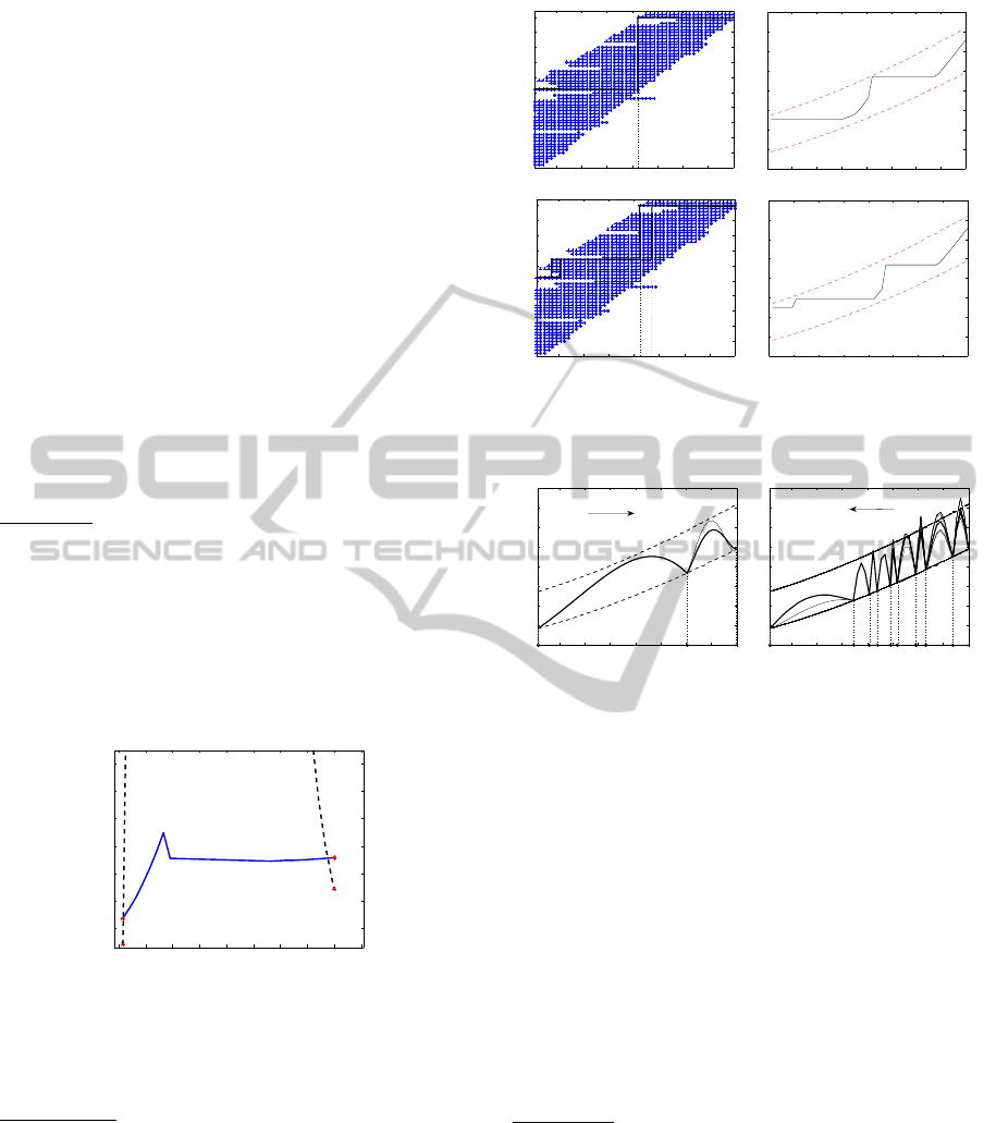
Figure 7 shows a simulation in closed-loop where
the scheduling function K(p) uses three robust con-
trollers K
rob
(p), and where p(t) increases within 1.2
sec from 720 to 780 and then decreases back to 710.
0 0.5 1 1.5 2 2.5
−1
0
1
x 10
−5
Perturbation rejection: w
2
=[1.3e−5sin(pt),1.3e−5cos(pt)]
0 0.5 1 1.5 2 2.5
720
740
760
780
t [s]
Rotor speed variation
K
rob
(707.5)
K
rob
(801.7)
K
rob
(707.5)
x
2
(a)
(b)
x
1
Figure 7: Simulation in closed loop. The scheduled pa-
rameter increases within 1.2 sec from 720 to 780, and de-
creases back to 710 within another 1.5 sec. Three con-
trollers K
rob
(p(t)) are called for. Upper image shows
unbalance compensation x
1
,x
2
for simulated w
2
(t) =
(1.3e− 5sin p(t), 1.3e− 5cos p(t)). (For x
1
,x
2
,w
2
see sec-
tion 3).
10 CONCLUSIONS
Several methods to compute a parameter varying de-
centralized PID for a magnetic bearing device were
compared. Performance was measured in the H
∞
norm, and the curve K
∗
(p) of optimal H
∞
-controllers
was taken as a reference to assess the performance
of the different parameterizations K(p). If parame-
terizations K(p) with a maximum loss of 10% over
K
∗
(p) were allowed, switching between piecewise
affine controllers on subintervals was found to per-
form best, but needs solving a mixed H
∞
/H
∞
synthe-
sis program. Interpolation based on computing vari-
ous K
∗
(p) was an interesting alternative, even though
it was observed that interpolation seems to have a
stronger tendency to lose stability and important de-
pendence at the beginning point. While the switching
technique carries over to 2D parameter sets, there is
no obvious way to extend interpolation into two di-
mensions.
ACKNOWLEDGEMENTS
This work was supported by research grants Techni-
com from Fondation d’Entreprise EADS, and Survol
from Fondation de Recherche pour l’A´eronautique et
l’Espace (FNRAE).
REFERENCES
Apkarian, P. and Gahinet, P. (1996). A convex characteriza-
tion of gain-scheduled H
∞
controllers. In IEEE Trans-
actions on Control Systems Technology, vol. 40, No. 5,
pp. 835-864.
Apkarian, P., Gahinet, P., and Becker, G. (1995). Self-
scheduled H
∞
control of linear parameter-varying sys-
tems: a design example. In Automatica, vol. 31, No.
9, pp. 1251-1261.
Chesi, G., Garulli, A., Tesi, A., and Vicino, A. (2009). Ho-
mogeneous polynomial forms for robustness analysis
of uncertain systems. In Springer Verlag.
Hinrichsen, D. and Pritchard, A. (1986a). Stability radii of
linear systems. In Systems and Control Letters, vol. 7,
pp. 1-10.
Hinrichsen, D. and Pritchard, A. (1986b). Stability radius
for structured perturbations and the algebraic riccati
equation. In Systems and Control Letters, vol. 8, pp.
105-113.
Hosseini-Ravanbod, L., Noll, D., and Apkarian, P. (2011a).
On a generalization of the LTR procedure. In Chinese
Control and Decision Conference, Mianyang, China.
Hosseini-Ravanbod, L., Noll, D., and Apkarian, P. (2011b).
Robustness via structured H
∞
/H
∞
-synthesis. In Inter-
national Journal of Control. In press.
Karow, M., Kokiopoulou, E., and Kressner, D. (2010).
On the computation of structured singular values and
pseudospectra. In Systems and Control Letters, vol.
59, No. 2, pp. 122-129.
Lanzon, A. and Tsiotras, P. (2005). A combined applica-
tion of H
∞
loop shaping and µ- synthesis to control
high-speed flywheels. In IEEE Transactions on Con-
trol Systems Technology, vol. 13, No. 5.
Lawrence, C., Tits, A. L., and Dooren, P. (2000). A fast
algorithm for the computation of an upper bound on
the µ-norm. In Automatica, vol. 36, pp. 449-456.
Mohamed, A. and Busch-Vishniac, I. (1995). Imbalance
compensation and automation balancing in magnetic
bearing systems using the q-parametrization theory.
In IEEE Transactions on Control Systems Technology,
vol. 3, No. 2.
Packard, A. (1994). Gain scheduling via linear fractional
transformations. In Systems and Control Letters, vol.
22, pp. 79-92.
Scherer, C. (2003). Higher-order relaxations for robust lmi
problems with verification for exactness. In Proceed-
ings of the 42nd IEEE Conference on Decision and
Control, pp. 4652 - 4657.
ICINCO 2011 - 8th International Conference on Informatics in Control, Automation and Robotics
336

Smith, R. and Weldon, W. (1995). Nonlinear control of
a rigid rotor magnetic bearing system: modeling and
simulation with full state feedback. In IEEE Transac-
tions on Magnetics, vol. 31, no. 2, pp. 973 - 980.
Tsiotras, P. and Mason, S. (1996). Self-sheduled H
∞
con-
trollers for magnetic bearings. In Proc. Int. Mechan-
ical Engineering Congr. Exposition, Atlanta, GA, pp.
151-158.
GAIN-SCHEDULED PID FOR IMBALANCE COMPENSATION OF A MAGNETIC BEARING
337