
AN INTERPOLATION APPROACH FOR CONSTRAINED
OUTPUT FEEDBACK
Hoai Nam Nguyen, Sorin Olaru
SUPELEC Systems Sciences (E3S), Automatic Control Department, Gif sur Yvette, France
Per-Olof Gutman
Faculty of Civil and Environmental Engineering, Technion - Israel Institute of Technology, Haifa, Israel
Morten Hovd
Department of Engineering Cybernetics, Norwegian University of Science and Technology, Trondheim, Norway
Keywords:
Output feedback, Controlled invariant set, Maximal admissible set, Constrained optimal control, Model pre-
dictive control.
Abstract:
The purpose of this paper is twofold. In the first part, we provide a solution to the problem of the state
construction through measurement and storage of appropriate previous measurements. In the second part we
consider the robust control problem of constrained discrete-time linear-time invariant systems with disturbance
and bounded input. Based on an interpolation technique, feasibility and a robustly asymptotically stable closed
loop behavior are guaranteed.
1 INTRODUCTION
This paper considers the problem of output feedback
control design for a class of linear discrete time sys-
tems in presence of output and control constraints and
subject to bounded disturbance. The boundedness as-
sumptions on the different manipulated signals will
be modeled by means of polyhedral constraints which
assure a global linear system description (linear dif-
ference equation and linear equalities/inequalities).
There are several papers in the literature dealing
with the output feedback synthesis problem. Due to
the presence of input and state constraints, the robust
model predictive control (MPC) design seems to best
fit our objectives. Indeed, based on a Luenberger ob-
server, an approach that incorporates the error on the
state estimation as an additive bounded disturbance
has been proposed in (Mayne et al., 2006). The esti-
mation error is then taken in to account in the classi-
cal design of the constrained controller. A different
approach is taken in (Goulart and Kerrigan, 2007),
where the authors include the observer dynamics in
the computation of the domain of attraction of the
closed loop system.
The main drawback of the observer-based ap-
proaches is that, when the constraints become active,
the nonlinearity dominates the properties of the state
feedback control system and one cannot expect the
separation principle to hold. Moreover there is no
guarantee that the constraints will be satisfied along
the closed-loop trajectories.
The work of (Wang and Young, 2006) proposed an
approach to MPC based on a non-minimal state space
model, in which the states are represented by mea-
sured past inputs and outputs. This approach elim-
inates the need of an observer. However the result-
ing state space model is unobservable and the state
dimension may be large.
The main aim of the present paper is twofold. In
the first part, we revisit the problem of state construc-
tion through measurement and storage of appropri-
ate previous measurements. We recall that, there ex-
ists a minimal state space model with the structural
constraints of having a state variable vector available
though measurement and storage of appropriate previ-
ous measurements. Even if this model might be non-
minimal from the classical state space representation
point of view, it is directly measurable and will pro-
5
Nam Nguyen H., Olaru S., Gutman P. and Hovd M..
AN INTERPOLATION APPROACH FOR CONSTRAINED OUTPUT FEEDBACK.
DOI: 10.5220/0003511900050013
In Proceedings of the 8th International Conference on Informatics in Control, Automation and Robotics (ICINCO-2011), pages 5-13
ISBN: 978-989-8425-74-4
Copyright
c
2011 SCITEPRESS (Science and Technology Publications, Lda.)

vide an appropriate model for the control design with
constraints handling guarantees.
In the second part, starting from this state space
model, we consider the robust control problem of con-
strained discrete-time linear invariant systems with
disturbance and bounded input. For this purpose, two
types of controller will be used in this paper. The
first one is the global vertex controller (Gutman and
Cwikel, 1986). The second one is the local uncon-
strained robust optimal control. Based on an inter-
polation technique and by minimizing an appropriate
objective function, feasibility and a robustly asymp-
totically stable closed loop behavior are achieved.
The following notations will be used throughout
the paper. We call a C-set a convex and compact set
and containing the origin as an interior point. A poly-
hedron, or a polyhedral set, is the intersection of a
finite number of half spaces. A polytope is a closed
and bounded polyhedral set. Given two sets X
1
⊂ R
n
and X
2
⊂ R
n
, the Minkowski sum of the sets X
1
and
X
2
is defined by X
1
⊕X
2
, {x
1
+x
2
| x
1
∈ X
1
, x
2
∈ X
2
}.
The set X
1
is a proper subset of the set X
2
if and only
if X
1
lies strictly inside X
2
. For the set X, let Fr(X) be
the boundary of X, Int(X) be the interior of X.
The paper is organized as follows. Section 2 is
concerned with the problem statement. Section 3
is dedicated to the state space realization. Section
4 deals with the problem of computing an invariant
set, while Section 5 is concerned with an interpola-
tion technique. The simulation results are evaluated
in Section 6 before drawing the conclusions.
2 PROBLEM STATEMENT
Consider the regulation problem for the followingdis-
crete linear time-invariant system, described by the
input-output relationship
y(t + 1) + D
1
y(t) + D
2
y(t − 1) + . . . + D
n
y(t − n+ 1)
= N
1
u(t) + N
2
u(t − 1) + . . . + N
m
u(t − m+ 1) + w(t)
(1)
where: y(t) ∈ R
q
, u(t) ∈ R
p
, w(t) ∈ R
q
and D
i
, i =
1, . . . , n and N
i
, i = 1, . . . , m are matrices of suitable
dimension.
It is assumed that m ≤ n.
The output and control are subject to the following
hard constraints
y(t) ∈ Y, u(t) ∈ U (2)
where Y = {y : F
y
y ≤ g
y
} and U = {u : F
u
u ≤ g
u
} are
polyhedral sets and contain the origin in their interior.
The signal w(t) represents the disturbance input.
In this paper, we assume that the disturbance w(t)
is unknown, additive and lie in the polytope W, i.e.
w(t) ∈ W, where W = {w : F
w
w ≤ g
w
} is a C-set.
3 STATE SPACE MODEL
In this section, the measured plant input, output and
their past measured values are used to represent the
states of the plant.
To simplify the description, it is assumed that
m = n. Note that this assumption is always true, by
supposing N
m+1
= N
m+2
= . . . = N
n
= 0.
The state of the system along the lines of (Taylor
et al., 2000). All the state construction is detailed such
that the presentation of the results to be self contained.
x(t) =
x
1
(t)
T
x
2
(t)
T
. . . x
n
(t)
T
T
(3)
where (∗)
T
denotes the transposed of matrix (∗) and
x
1
(t) = y(t)
x
2
(t) = −D
n
x
1
(t − 1) + N
n
u(t − 1)
x
3
(t) = −D
n−1
x
1
(t − 1)+ x
2
(t − 1) + N
n−1
u(t − 1)
x
4
(t) = −D
n−2
x
1
(t − 1)+ x
3
(t − 1) + N
n−2
u(t − 1)
.
.
.
x
n
(t) = −D
2
x
1
(t − 1) + x
n−1
(t − 1) + N
2
u(t − 1)
(4)
It is clear that
x
2
(t) = −D
n
y(t − 1) +N
n
u(t − 1)
x
3
(t) = −D
n−1
y(t − 1) − D
n
y(t − 2)+
+ N
n−1
u(t − 1) + N
n
u(t − 2)
.
.
.
x
n
(t) = −D
2
y(t − 1) −D
3
y(t − 2) − . . . − D
n
y(t − n+1)+
+ N
2
u(t − 1) + N
3
u(t − 2) + . . . + N
n
u(t − n+ 1)
One has
y(t + 1) = −D
1
y(t)− D
2
y(t − 1) −. . . −D
n
y(t − n+ 1)
+N
1
u(t)+N
2
u(t − 1) + . . . + N
n
u(t − n+ 1)+ w(t)
or
x
1
(t + 1) = −D
1
x
1
(t) + x
n
(t) + N
1
u(t)+w(t)
The state space model is then defined as follows
x(t + 1) = Ax(t)+ Bu(t)+ Ew(t)
y(t) = Cx(t)
(5)
where
A =
−D
1
0
q
0
q
. . . 0
q
I
q
−D
n
0
q
0
q
. . . 0
q
0
q
−D
n−1
I
q
0
q
. . . 0
q
0
q
−D
n−2
0
q
I
q
. . . 0
q
0
q
. . . . . . . . . . . . . . . . . .
−D
2
0
q
0
q
. . . I
q
0
q
,
B =
N
T
1
N
T
n
N
T
n−1
N
T
n−2
. . . N
T
2
T
,
E =
I
q
0
q
0
q
0
q
. . . 0
q
T
,
C =
I
q
0
q
0
q
0
q
. . . 0
q
.
ICINCO 2011 - 8th International Conference on Informatics in Control, Automation and Robotics
6

Here I
q
, 0
q
denote the identity and zeros matrices of
dimension q× q, respectively.
It should be noted that, the state space realization
(5) is minimal in the single input single output case.
In the other cases this realization might not be mini-
mal, as showing in the following example.
Consider the SIMO discrete time system:
y(t + 1) +
−2 0
0 −2
y(t)+
1 0
0 1
y(t − 1) =
=
0.5
2
u(t)+
0.5
1
u(t − 1) + w(t)
(6)
Using the above construction, the state space
model is given as follows:
x(t + 1) = Ax(t) + Bu(t) + Ew(t)
y(t) = Cx(t)
where
A =
2 0 1 0
0 2 0 1
−1 0 0 0
0 −1 0 0
, B =
0.5
0.5
0.5
−1.5
E =
1
1
0
0
, C =
1 0 0 0
0 1 0 0
It is obvious that, this realization is not minimal. One
of the minimal realizations of the system is given by:
A =
0 −1
1 2
, B =
0.5
0.5
, E =
0
1
C =
0 1
1 0
Denote
z(t) = (y(t)
T
y(t − 1)
T
. . . y(t − n+ 1)
T
u(t − 1)
T
u(t − 2)
T
. . . u(t − n+ 1)
T
)
T
(7)
The state vector x(t) (3) is related to the vector z(t)
as follows
x(t) = Tz(t) (8)
where
T = (T
1
T
2
)
T
1
=
I
q
0
q
0
q
. . . 0
q
0
q
−D
n
0
q
. . . 0
q
0
q
−D
n−1
−D
n
. . . 0
q
. . . . . . . . . . . . . . .
0
q
−D
2
−D
3
. . . −D
n
T
2
=
0
q×p
0
q×p
0
q×p
. . . 0
q×p
N
n
0
q×p
0
q×p
. . . 0
q×p
N
n−1
N
n
0
q×p
. . . 0
q×p
. . . . . . . . . . . . . . .
N
2
N
3
N
4
. . . N
n
From the formula (8), it is apparent that at any
time instant t, the state variable vector is available
though measurement and storage of appropriate pre-
vious measurements.
4 INVARIANT SET
CONSTRUCTION
Using (4), it is clear that x
i
(t) ∈ X
i
where X
i
is given
by
X
1
= Y
X
2
= D
n
(−X
1
) ⊕ N
n
(U)
X
i
= D
n+2−i
(−X
1
) ⊕ X
i−1
⊕ N
n+2−i
U, ∀i = 3, . . . , n
In summary, the constraints on the state are x ∈ X,
where X = {x : F
x
x ≤ g
x
}.
4.1 Maximal Robustly Admissible Set
for u = Kx
Using the results in the control theory (LQR, LQG,
LMI based, . . .), one can find a feedback gain K, that
quadratically stabilizes the system (5) with some de-
sired properties. The details of such a synthesis pro-
cedure are not reproduced here, but we assume that
the feasibility of such an optimization based robust
control design is guaranteed, leading to a closed loop
transition matrix A
c
= A+ BK.
Definition 1 (Robustly Positively Invariant Set).
The set Ω ⊆ X is a robustly positively invariant (RPI)
set with respect to x(t + 1) = A
c
x(t) + Ew(t) if and
only if
∀x ∈ Ω ⇒ A
c
x+ Ew ∈ Ω (9)
for any w ∈ W.
Definition 2 (Minimal RPI). The set Ω
∞
⊆ X is a
minimal RPI (mRPI) set with respect to x(t + 1) =
A
c
x(t) + Ew(t) if and only if Ω
∞
is a RPI and con-
tained in any RPI set.
It is possible to show that if the mRPI set Ω
∞
ex-
ists, then it is unique, bounded and contains the ori-
gin in its interior (Kolmanovsky and Gilbert, 1998),
(Rakovic et al., 2005). Moreover, all trajectories of
the system x(t + 1) = A
c
x(t) + Ew(t) starting from
the origin, are bounded by Ω
∞
. It follows from lin-
earity and asymptotic stability of A
c
, that Ω
∞
is the
limit set of all trajectory of the system x(t + 1) =
A
c
x(t) + Ew(t).
It is clear that, it is impossible to devise a con-
troller u(t) = Kx(t) such that x(t) → 0 as t → ∞. The
best that can be hoped for is that the controller steers
any initial state to the mRPI set Ω
∞
, and maintains the
AN INTERPOLATION APPROACH FOR CONSTRAINED OUTPUT FEEDBACK
7

state in this set once it is reached. In other words, the
set Ω
∞
can be considered as the origin of the system
(5).
In the sequel, it is assumed that the set Ω
∞
is a
proper subset Y.
Definition 3 (Maximal RPI). The set O
∞
∈ X is a
maximal RPI (MRPI) set with respect to x(t + 1) =
A
x
x(t)+Ew(t) if and only if O
∞
is a RPI and contains
every RPI set.
If the MRPI set is non-empty, then it is unique.
Furthermore if X,U andW are a C-set, then the MRPI
set O
∞
is also a C-set.
The mRPI set Ω
∞
and the MRPI set O
∞
are con-
nected be the following theorem:
Theorem 1. The following statements are equiva-
lent:
1. The MRPI set O
∞
is non-empty.
2. Ω
∞
⊂ X
Proof. Interested readers are referred to (Kol-
manovsky and Gilbert, 1998) for the details of the
proof.
Define the polytope P
xu
as follows
P
xu
= {x : F
xu
x ≤ g
xu
} (10)
where
F
xu
=
F
x
F
u
K
, g
xu
=
g
x
g
u
Under the assumption that the Ω
∞
is a proper sub-
set of X, a constructive procedure is used to compute
the MRPI set, as follows (Blanchini and Miani, 2008).
Procedure 1. Maximal robustly positively invariant
set computation.
1. Set t = 0, F
t
= F
xu
, g
t
= g
xu
and P
t
= P
xu
.
2. Set P
1
t
= P
t
3. Solve the following linear program
d = maxF
t
Ew, s.t. w ∈ W
4. Compute a polytope
P
2
t
= {x : F
t
A
c
x ≤ g
t
− d}
5. Set P
t
as an intersection
P
t
= P
1
t
∩ P
2
t
6. If P
t
= P
1
t
then stop and set O
∞
= P
t
. Else con-
tinue.
7. Set t = t + 1, go to step 2.
Non-emptiness property of the MRPI set O
∞
as-
sures that the above procedure terminates in finite
time and lead to the MRPI in form of a polytope
O
∞
= {x : F
o
x ≤ g
o
} (11)
4.2 Robustly Positively Controlled
Invariant Set for u ∈ U
Recall the followingdefinitions (Blanchini and Miani,
2008)
Definition 4: Robustly Positively Controlled In-
variant Set. Given the system (5), the set Ψ ⊆ X
is invariant if and only if for any x(t) ∈ Ψ, there exists
a control action u(t) ∈ U such that for any w(t) ∈ W,
one has x(t + 1) = Ax(t) + Bu(t) + Ew(t) ∈ X.
Definition 5: Pre-image Set. Given the polytopic
system (1), the one-step pre-image set of the set P
0
=
{x : F
0
x ≤ g
0
} is given by all states that be steered in
one step in P
0
when a suitable control is applied. The
pre-image set, called P
1
= Pre(P
0
) can be shown to
be:
P
1
= {x∈ R
n
:∃u ∈ U : F
0
(Ax+Bu) ≤ g
0
−maxF
0
Ew}
(12)
where w ∈ W.
Remark 1: It is clear that if the set Ψ is contained
in its pre-image set the Ψ is invariant.
Recall that the set O
∞
is the MRPI. Define P
N
as
the set of states, that can be steered to the O
∞
in no
more that N steps along an admissible trajectory, i.e.
a trajectory satisfying control, state and disturbance
constraints. This set can be generated recursively by
the following procedure:
Procedure 2. Invariant set computation
1. Set k = 0 and P
0
= O
∞
.
2. Define
P
k+1
= Pre(P
k
)
\
X
3. If P
k+1
= P
k
, then stop and set P
N
= P
k
. Else con-
tinue.
4. If k = N, then stop else continue.
5. Set k = k+ 1 and go to the step 2.
A a consequence of the fact that O
∞
is an invariant
set, it follows that for each k, P
k−1
⊂ P
k
and therefore
P
k
is an invariant set and a sequence of nested poly-
topes.
Note that the complexity of the set P
N
does not
have an analytic dependence on N and may increase
without bound, thus placing a practical limitation on
the choice of N.
For further use, the controlled invariant set result-
ing from the Procedure 2 is denoted
P
N
= {x : F
N
x ≤ g
N
} (13)
ICINCO 2011 - 8th International Conference on Informatics in Control, Automation and Robotics
8

5 INTERPOLATION BASED
CONTROLLER WITH LINEAR
PROGRAMMING
The purpose of this section is to show how an inter-
polation technique can be used together with linear
programming.
5.1 Vertex Control Law
Given a positve invariant polytope P
N
∈ R
n
, this poly-
tope can be decomposed in a sequence of simplices
P
k
N
each formed by n vertices x
(k)
1
, x
(k)
2
, . . . , x
(k)
n
and the
origin. These simplices have following properties:
• Int(P
k
N
) 6=
/
0,
• Int(P
k
N
∩ P
l
N
) =
/
0 if k 6= l,
•
S
k
P
k
N
= P
N
,
Denote by X
(k)
= (x
(k)
1
x
(k)
2
. . . x
(k)
n
) the square ma-
trix defined by the vertices generating P
k
N
. Since P
k
N
has nonempty interior, X
(k)
is invertible. Let U
(k)
=
(u
(k)
1
u
(k)
2
. . . u
(k)
n
) be the matrix defined by the admis-
sible control values at these vertices. For x ∈ P
k
N
con-
sider the following linear gain K
k
:
K
k
= U
(k)
(X
(k)
)
−1
(14)
Remark 2: By the admissible control value we under-
stand any control action, that keeps the state inside
the invariant set. Generally, one would like to maxi-
mize the control action at the vertices of the feasible
invariant set. This can be done by using the following
program.
J = maxkuk
p
s.t.
F
N
(Ax+ Bu) ≤ g
N
− maxF
N
Ew
F
u
u ≤ g
u
.
(15)
where kuk
p
is a p− norm of u and w ∈ W.
Due to the properties of the positive invariant set,
the above program is always feasible.
Theorem 2. The piecewise linear control u = K
k
x is
feasible and asymptotically stable for all x ∈ P
N
.
Proof. The proof of this theorem is not reported
here, with (Gutman and Cwikel, 1986) and (Blan-
chini, 1992) providing the necessary details.
5.2 Interpolation via Linear
Programming
Any state x(t) in P
N
can be decomposed as follows:
x(t) = cx
v
(t) + (1 − c)x
o
(t) (16)
where x
v
(t) ∈ P
N
, x
o
(t) ∈ Ω and 0 ≤ c ≤ 1.
Consider the following control law:
u(t) = cu
v
(t) + (1 − c)u
o
(t) (17)
where u
v
(t) is obtained by applying the vertex con-
trol law and u
o
(t) = Kx
o
(t) is the control law, that is
feasible in O
∞
.
Figure 1: Feasible regions for example 1. The blue one is
the MRPI O
∞
, when applying the control law u = Kx. The
red one is the positive invariant set P
N
.
Theorem 3. The above linear control is feasible
for all x ∈ P
N
.
Proof.
Corresponding to the decomposition, the control
law is given by (17).
One has to prove that F
u
u(t) ≤ g
u
and x(t + 1) =
Ax(t) + Bu(t) + Ew(t) ∈ P
N
for all x(t) ∈ P
N
and for
any w(t) ∈ W .
One has
F
u
u(t) = F
u
(cu
v
(t) + (1 − c)u
o
(t))
= cF
u
u
v
(t) + (1 − c)F
u
u
o
(t)
≤ cg
u
+ (1− c)g
u
= g
u
and
x(t + 1) = Ax(t) + Bu(t) + Ew(t)
= A(cx
v
(t) + (1 − c)x
o
(t))+
+ B(cu
v
(t) + (1 − c)u
o
(t)) + Ew(t)
= c(Ax
v
(t) + Bu
v
(t) + Ew(t))+
+ (1− c)(Ax
o
(t) + Bu
o
(t) + Ew(t))
We have Ax
v
(t) + Bu
v
(t) + Ew(t) ∈ P
N
and
Ax
o
(t) + Bu
o
(t) + Ew(t) ∈ O
∞
⊂ P
N
, it follows that
x(t + 1) ∈ P
N
.
In order to give a maximal control action, one
would like to minimize c, so the following program
is given:
c
∗
(x) = min
c,x
v
,x
o
c, s.t.
F
N
x
v
≤ g
N
,
F
o
x
o
≤ g
o
,
cx
v
+ (1− c)x
o
= x,
0 ≤ c ≤ 1
(18)
AN INTERPOLATION APPROACH FOR CONSTRAINED OUTPUT FEEDBACK
9

Denote r
v
= cx
v
, r
o
= (1 − c)x
o
. It is clear that
r
v
∈ cP
N
and r
o
∈ (1−c)Ω or equivalently F
N
r
v
≤ cg
N
and F
w
r
o
≤ (1− c)g
w
. The above non-linear program
is translated into a linear program as follows.
Interpolation based on Linear Programming.
c
∗
(x) = min
c,r
v
c, s.t.
F
N
r
v
≤ cg
N
F
o
(x− r
v
) ≤ (1− c)g
o
0 ≤ c ≤ 1
(19)
Remark 3. If one would like to maximize c, it is
obvious that c = 1 for all x ∈ P
N
. In this case the
controller turns out to be the vertex controller.
Theorem 4. The control law using interpolation
based on linear programming (16), (17), (19) guar-
antees robustly asymptotic stability for all initial state
x(0) ∈ P
N
.
Proof. The complete proof of this theorem is
given in (Nguyen et al., 2011).
6 EXAMPLES
To show the effectiveness of the proposed approach,
two examples will be presented in this section. For
both of these examples, to solve linear programs
and to implement polyhedral operations, we used the
Multi-parametric toolbox, (Kvasnica et al., 2004).
6.1 Example 1
Consider the following discrete-time system
y(t + 1) −2y(t)+ y(t −1) =
= 0.5u(t)+ 0.5u(t − 1) + w(t)
(20)
The constraints are
−5 ≤ y(t) ≤ 5
−5 ≤ u(t) ≤ 5
and
−0.1 ≤ w(t) ≤ 0.1
The state space model is given by
x(t + 1) = Ax(t) + Bu(t) + Ew(t)
y(t) = Cx(t)
where
A =
2 1
−1 0
, B =
0.5
0.5
, E =
1
0
,
and
C =
1 0
The state x(t) is available though the measured
plant input, output and their past measured values as
follows
x(t) = Tz(t)
where
z(t) =
y(t) y(t − 1) u(t − 1)
T
,
T =
1 0 0
0 −1 0.5
The constraints on the state are
−5 ≤ x
1
≤ 5
−7.5 ≤ x
2
≤ 7.5
Using the linear quadratic regulator with weight-
ing matrices Q = C
′
C and R = 0.1 the feedback gain
is obtained
K =
−2.3548 −1.3895
Using procedures 1 and 2 one obtains the set O
∞
and P
N
as shownin Figure 1. Note that P
3
= P
4
, in this
case P
3
is a maximal invariant set for system (20).
The set of vertices of P
N
is given by the matrix
V(P
N
) below, together with the control matrix U
v
V(P
N
) =
−5 −0.1 5 0.1 −0.1 −5 0.1 5
7.5 7.5 −2.6 7.2 −7.2 2.6 −7.5 −7.5
and
U
v
=
−5 −5 −5 −4.9 5 5 5 4.9
Figure 2 shows the state space partition and 6 dif-
ferent trajectories of the closed loop system.
Figure 2: State space partition and trajectories of the closed
loop system for example 1.
Corresponding to the initial condition x
0
=
(5.0000 − 2.6000)
T
, Figure 3 shows the output and
input trajectory.
Figure 4 shows the disturbance input and the in-
terpolating coefficient c
∗
(t) as a function of t. As ex-
pected this function is positive and non-increasing.
In a comparison with the approach, that based on
the so called Kalman filter, Figure 5 shows the output
ICINCO 2011 - 8th International Conference on Informatics in Control, Automation and Robotics
10
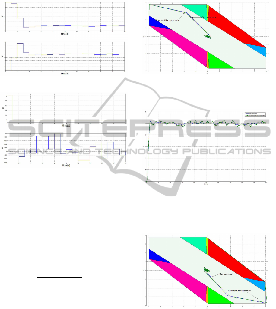
Figure 3: Output and input trajectory for example 1.
Figure 4: The interpolating coefficient and the disturbance
input for example 1.
trajectories using our approach and the Kalman filter
based approach. It is obvious that, the mRPI set of the
Kalman filter based approach is bigger than the mRPI
set of our approach.
The Matlab routine with the command ’kalman’
is used for designing the Kalman filter. The process
noise is a white noise with an uniform distribution and
there is no measurement noise.
w is a random number with an uniform distribu-
tion, w
l
≤ w ≤ w
u
. The variance of w is given as fol-
lows:
C
w
=
(w
u
− w
l
+ 1)
2
− 1
12
= 0.0367
The estimator gain of the Kalman filter is ob-
tained:
L = (2 − 1)
T
The initial condition is x
0
= (−4 6)
T
.
The Kalman filter is used to estimate the state of
the system and then this estimation is used to close
the loop with the interpolated control law .
In contrast to our approach, where the state is ex-
act, in the Kalman filter approach, the state is not ex-
act and moreover, there is no guarantee that the con-
straints are satisfied.
Figure 6 shows the output trajectories of our ap-
proach and the Kalman filter based approach.
Figure 5: The state trajectory of our approach and the
Kalman filter based approach for example 1. The mRPI set
of the Kalman filter based approach is bigger than the mRPI
set of our approach.
Figure 6: The output trajectories of our approach and the
Kalman filter based approach for example 1.
In Figure 7 it is showed that, the constraints might
be violated where the Kalman filter is used to estimate
the state of the system.
Figure 7: Constraints violation for example 1.
6.2 Example 2
Consider the following discrete-time system
y(t + 1) +
−1.8787 0
0 −1.8964
y(t)+
+
0.8787 0
0 0.8964
y(t − 1) =
AN INTERPOLATION APPROACH FOR CONSTRAINED OUTPUT FEEDBACK
11
=
−0.3800 −0.5679
−0.2176 0.4700
u(t)+
+
0.3339 0.5679
0.2176 −0.4213
u(t − 1) + w(t)
(21)
The constraints are
−2 ≤ y
1
≤ 2, − 2 ≤ y
2
≤ 2
−10 ≤ u
1
≤ 10, − 10 ≤ u
2
≤ 10
and
−0.1 ≤ w
1
≤ 0.1, − 0.1 ≤ w
2
≤ 0.1
The state space model is
x(t + 1) = Ax(t) + Bu(t) + Ew(t)
y(t) = Cx(t)
where
A =
1.8787 0 1.000 0
0 1.8964 0 1
−0.8787 0 0 0
0 −0.8964 0 0
,
B =
−0.3800 −0.5679
−0.2176 0.4700
0.3339 0.5679
0.2176 −0.4213
, E =
1 0
0 1
0 0
0 0
C =
1 0 0 0
0 1 0 0
It is worth noticing that, the above state space re-
alization is minimal. The state x(t) is availablethough
the measured plant input, output and their past mea-
sured values as follows
x(t) = Tz(t)
where
z(t) =
y(t)
T
y(t − 1)
T
u(t − 1)
T
T
,
T =
1.0 0 0 0 0 0
0 1.0 0 0 0 0
0 0 −0.8787 0 0.3339 0.5679
0 0 0 −0.8964 0.2176 −0.4213
The constraints on the state are
1 0 0 0
0 1 0 0
−1 0 0 0
0 −1 0 0
0 0 0.5460 −0.8378
0 0 −0.5958 −0.8031
0 0 −1.0000 0
0 0 −0.5460 0.8378
0 0 0 1.0000
0 0 0.0000 −1.0000
0 0 0.5958 0.8031
0 0 1.0000 0.0000
x ≤
2
2
2
2
9.0918
6.2239
10.7754
9.0918
8.1818
8.1818
6.2239
10.7754
Using the linear quadratic regulator with weight-
ing matrices Q = C
′
C and R = I, the feedback gain is
obtained
K =
1.9459 1.7552 1.4968 1.3775
0.8935 −1.7212 0.5524 −1.2704
Using procedures 1 and 2, one obtains the set
O
∞
and P
3
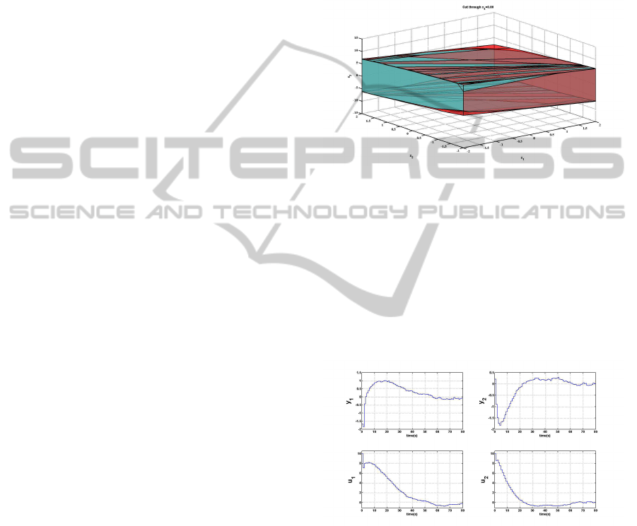
as illustrated in Figure 8. The num-
Figure 8: Feasible regions for example 2, cut through x
4
=
0. The blue one is the MRPI set O
∞
, when applying the
control law u = Kx. The red one is the positive controlled
invariant set P
3
.
ber of vertices of the set P
3
is 1030 and these are
not reported here. The control values at the ver-
tices of the set P
3
are found by applying the pro-
gram (15). Corresponding to the initial condition
x
0
=
−1.6722 0.2088 10.7754 −3.8296
T
,
Figure 9 presents the output and input trajectories.
Figure 9: Output and input trajectory for example 2.
Figure 10 shows the disturbance inputs
w
1
(t), w
2
(t) and the interpolating coefficient c
∗
(t) as
a function of t. As expected, this function is positive
and non-increasing.
In a comparison with the Kalman filter based ap-
proach, Figure 11 shows the output trajectories using
our approach and the Kalman filter based approach.
The initial condition is x
0
=
−1.3378 0.1670 8.6203 −3.0637
T
.
The Matlab routine with the command ’kalman’
is used for designing the Kalman filter. The process
ICINCO 2011 - 8th International Conference on Informatics in Control, Automation and Robotics
12

Figure 10: The interpolating coefficient and the disturbance
input for example 2.
noise is a white noise with an uniform distribution and
there is no measurement noise.
w is a random vector with an uniform distribution,
w
l
≤ w ≤ w
u
. The covariance matrix of w is given as
follows:
C
w
=
(w
u
−w
l
+1)
2
−1
12
1 0
0 1
=
0.0367 0
0 0.0367
The estimator gain of the Kalman filter is ob-
tained:
L =
1.8787 0
0 1.8964
−0.8787 0
0 −0.8964
Figure 11: The output trajectories of our approach and the
Kalman filter based approach for example 2.
7 CONCLUSIONS
In this paper, a state space realization is detailed for
discrete-time linear time invariant systems, with the
particularity that the state variable vector is available
through measurement and storage of appropriate pre-
vious measurements.
A robust control problem is solved based on the
interpolation technique and using linear program-
ming. Practically, the interpolation is done between
a global vertex controller and a local unconstrained
robust optimal control law.
Several simulation examples are presented includ-
ing a comparison with an earlier solution from the lit-
erature and a multi-input multi-output system.
REFERENCES
Blanchini, F. (1992). Minimum-time control for uncer-
tain discrete-time linear systems. In Proceedings of
the 31st IEEE Conference on Decision and Control,
1992., pages 2629–2634.
Blanchini, F. and Miani, S. (2008). Set-theoretic methods in
control. Springer.
Goulart, P. and Kerrigan, E. (2007). A method for robust re-
ceding horizon output feedback control of constrained
systems. In Decision and Control, 2006 45th IEEE
Conference on, pages 5471–5476. IEEE.
Gutman, P. and Cwikel, M. (1986). Admissible sets and
feedback control for discrete-time linear dynamical
systems with bounded controls and states. IEEE trans-
actions on Automatic Control, 31(4):373–376.
Kolmanovsky, I. and Gilbert, E. (1998). Theory and com-
putation of disturbance invariant sets for discrete-time
linear systems. Mathematical Problems in Engineer-
ing, 4(4):317–363.
Kvasnica, M., Grieder, P., Baotic, M., and Morari, M.
(2004). Multi-parametric toolbox (MPT). Hybrid Sys-
tems: Computation and Control, pages 121–124.
Mayne, D., Rakovic, S., Findeisen, R., and Allgower, F.
(2006). Robust output feedback model predictive
control of constrained linear systems. Automatica,
42(7):1217–1222.
Nguyen, H.-N., Gutman, P.-O., Olaru, S., Hovd, M., and
Colledani, F. (2011). Improved vertex control for un-
certain linear discrete-time systems with control and
state constraints. In American Control Conference,
2011. IEEE.
Rakovic, S., Kerrigan, E., Kouramas, K., and Mayne, D.
(2005). Invariant approximations of the minimal ro-
bust positively invariant set. Automatic Control, IEEE
Transactions on, 50(3):406–410.
Taylor, C., Chotai, A., and Young, P. (2000). State space
control system design based on non-minimal state-
variable feedback: further generalization and uni-
fication results. International Journal of Control,
73(14):1329–1345.
Wang, L. and Young, P. (2006). An improved struc-
ture for model predictive control using non-minimal
state space realisation. Journal of Process Control,
16(4):355–371.
AN INTERPOLATION APPROACH FOR CONSTRAINED OUTPUT FEEDBACK
13
