
TRANSFORMING ATTRIBUTE AND CLONE-ENABLED
FEATURE MODELS INTO CONSTRAINT PROGRAMS
OVER FINITE DOMAINS
Raúl Mazo
CRI, Panthéon Sorbonne University, 90, rue de Tolbiac, 75013 Paris, France
Departamento de Ingeniería de Sistemas, Universidad de Antioquia, Medellín, Colombia
Camille Salinesi, Daniel Diaz
CRI, Panthéon Sorbonne University, 90, rue de Tolbiac, 75013 Paris, France
Alberto Lora-Michiels
Baxter International Inc., Lessines, Belgium
Keywords: Requirement engineering, Product line models, Feature models, Transformation, Constraint programming.
Abstract: Product line models are important artefacts in product line engineering. One of the most popular languages to
model the variability of a product line is the feature notation. Since the initial proposal of feature models in
1990, the notation has evolved in different aspects. One of the most important improvements allows specify
the number of instances that a feature can have in a particular product. This improvement implies an
important increase on the number of variables needed to represent a feature model. Another improvement
consists in allowing features to have attributes, which can take values on a different domain than the
boolean one. These two extensions have increased the complexity of feature models and therefore have
made more difficult the manually or even automated reasoning on feature models. To the best of our
knowledge, very few works exist in literature to address this problem. In this paper we show that reasoning on
extended feature models is easy and scalable by using constraint programming over integer domains. The aim
of the paper is double (a) to show the rules for transforming extended feature models into constraint programs,
and (b) to demonstrate, by means of 11 reasoning operations over feature models, the usefulness and benefits
of our approach. We evaluated our approach by transforming 60 feature models of sizes up to 2000 features
and by comparing it with 2 other approaches available in the literature. The evaluation showed that our
approach is correct, useful and scalable to industry size models.
1 INTRODUCTION
Requirements Engineering is the process of
discovering system purpose by identifying
stakeholders and their needs, and documenting these
in a way that is amenable to reasoning,
communication, and subsequent implementation
(Nuseibeh and Easterbrook, 2000). When this
process is achieved in the context of Product Lines
(PL), its complexity and difficulty is much higher
since there are several products to consider, which
imply to manage the relationships of communality
and variability between them. One of the most
popular notations to specify the common and
variable requirements of a software product line is
the Feature Models (FMs). In the context of PLs,
FMs are used for product derivation, variability
reasoning and code generation (Kang et al., 1990),
(Van Deursen and Klint, 2002). In these contexts,
FMs are usually transformed to executable code in
order to reason on them (Batory, 2005), (Benavides
et al., 2005), (Benavides et al., 2007), (Benavides et
al., 2010), (Van Deursen and Klint, 2002), (Karataş et
al. 2010), (Salinesi et al., 2010). Since their first
introduction in 1990 as a part of the Feature-
Oriented Domain Analysis (FODA) method (Kang et
188
Mazo R., Salinesi C., Diaz D. and Lora-Michiels A..
TRANSFORMING ATTRIBUTE AND CLONE-ENABLED FEATURE MODELS INTO CONSTRAINT PROGRAMS OVER FINITE DOMAINS.
DOI: 10.5220/0003509301880199
In Proceedings of the 6th International Conference on Evaluation of Novel Approaches to Software Engineering (ENASE-2011), pages 188-199
ISBN: 978-989-8425-57-7
Copyright
c
2011 SCITEPRESS (Science and Technology Publications, Lda.)

al., 1990), several extensions have been proposed to
improve and enrich the expressiveness of FMs. The
first one was the introduction in the basic FODA
notation of cross-tree dependencies (requires and
excludes), to put constraints on features. The second
and the third extensions consisted in the introduction
of attributes (Diaz and Codognet, 2001), (Benavides
et al. 2005b) and cardinalities (feature and group
cardinalities) (Czarnecki et al. 2005), (Djebbi and
Salinesi, 2007), (Van Hentenryck, 1989). FMs with
these three extensions are called extended feature
models. Despite their pertinence for the industry,
most of the reasoning approaches on FMs do not
consider the last two extensions, or at best partially
(Benavides et al., 2010). In this paper we propose an
approach based on constraint programming that fills
this gap by handling reasoning on extended FMs.
In the last few years, Constraint Programming
(CP) has attracted attention among experts from
many areas because of its potential for solving hard
real life problems. Not only it is based on a strong
theoretical foundation but it is also attracting a
widespread commercial interest as well, in
particular, in areas of modelling heterogeneous
optimisation and satisfaction problems. In the PL
domain, several authors have proposed to use CP to
represent FMs but without attributes and
cardinalities (Batory, 2005), (Benavides et al., 2005)
or with lacks on quality representation and
implementation (Karataş et al., 2010).
The approach presented in this paper uses
constraint programming to represent extended
feature models with the purpose of reasoning on
them by using an existing constraint solver. Details
about reasoning operations on FMs are out of scope
of this paper. We begin describing extended feature
models and developing a relevant example to
illustrate the transformation process of extended
FMs into constraint programs and the subsequent
reasoning operations that can be executed on them.
We finally present an initial evaluation of our
approach. In our evaluation we transform to CP 60
feature models of sizes up to 2000 features. This
transformation has been compared with two other
approaches from the literature. The results obtained
by this experiment show that our approach is
pertinent because it fixes errors of one of the
existing approaches. The results also show that our
approach is (i) scalable to important size models,
which can be transformed into CPs in only few
seconds; and (ii) correct, compared with the already
state of the art approaches (Benavides 2007),
(Mendoça et al., 2009). We conclude the paper with
a discussion of related works, then of open issues
and we conclude with an outlook on future works.
2 BACKGROUND AND
MOTIVATION
2.1 Extended Feature Models
A FM defines the valid combinations of features in a
SPL, and is depicted as a graph-like structure in
which nodes represent features, and edges the
relationships between them (Kang et al., 2002). A
feature is a prominent or distinctive user-visible
aspect, quality, or characteristic of a software system
(Kang et al., 1990). A feature can have zero or more
attributes (Van Deursen and Klint, 2002), (Ziadi et
al., 2003). Cardinality-based feature models
(Czarnecki et al., 2005) allow specifying individual
cardinalities for each feature and group cardinalities
grouping bundles of features. In this paper, we use
the semantic of feature models proposed by
(Schobbens et al., 2007) and cardinality-based
feature models proposed by (Michel et al., 2011).
Components of a FM can be related among them by
means of the following relationships:
• Feature cardinality: Is represented as a sequence
of intervals [min..max] determining the
number of instances of a particular feature that
can be part of a product. Each instance is called a
clone.
• Attribute: Although there is no consensus on a
notation to define attributes, most proposals agree
that an attribute is a variable with a name, a
domain, and a value (consistent with the domain)
at a given configuration time.
• Father-child relationship, there are two kinds:
o Mandatory: Given two features F1 and F2,
F1 father of F2, a mandatory relationship
between F1 and F2 means that if the F1 is
selected, then F2 must be selected too and
vice versa.
o Optional: Given two features F1 and F2, F1
father of F2, an optional relationship between
F1 and F2 means that if F1 is selected then
F2 can be selected or not. However, if F2 is
selected, then F1 must also be selected.
o Requires: Given two features F1 and F2, F1
requires
F2 means that if F1 is selected in
product, then F2 has to be selected too.
Additionally, it means that F2 can be selected
even when F1 is not.
TRANSFORMING ATTRIBUTE AND CLONE-ENABLED FEATURE MODELS INTO CONSTRAINT PROGRAMS
OVER FINITE DOMAINS
189

o Exclusion: Given two features F1 and F2,
F1 excludes F2 means that if F1 is selected
then F2 cannot to be selected in the same
product. This relationship is bi-directional: if
F2 is selected, then F1 cannot to be selected
in the same product.
• Group cardinality: A group cardinality is an
interval denoted <n..m>, with n as lower bound
and m as upper bound limiting the number of
child features that can be part of a product when
its parent feature is selected. If one of the child
features is selected, then the father feature must
be selected too.
As a running example, we illustrate cardinality
and non-cardinality based feature models with a
hypothetical case of a Movement Control System
(MCS) of a car. This example is a simplified extract
of a real FM developed with one of our industrial
partners. A more complete extract of the model is
explained in (Salinesi et al., 2010b) and (Salinesi et
al., 2011). In Figure 1, we present the cardinality-
based FM of the allocation of hardware resources for
a car MCS. A MCS is composed of one or several
sensors, one or two processors and one or two slots
of internal memory. Sensors are used to measure the
speed and position of a car by means of two features
called Speed Sensor
and Position Sensor,
respectively. Speed Sensor is represented as a
mandatory feature (with a feature cardinality
[1..1]). And Position Sensor is represented
as an optional feature (with a feature cardinality
[0..4]). These two features are related by means
of a requires relationship. To compute the location
of a car, the MCS uses one or two processors, each
one associated by means of a mandatory relationship
with one or two slots of
Internal Memory.
Internal memory can take the values of 128, 512 or
1024 as specified in its attribute Size
.
S
p
eedSensor
Movement Control System
PositionSensor
Processor
[0..4]
[1..1]
[1..2]
Internal Memor
y
[1..2]
Size:{128,512,1024}
Figure 1: Example of feature model. Extract of an
allocation of resources for a movement control system of a
car.
2.2 Constraint Programming
in a Nutshell
Constraint Programming (CP) emerged in the 1990’s
as a successful paradigm to tackle complex
combinatorial problems in a declarative manner
(Van Hentenryck, 1989). CP extends programming
languages with the ability to deal with logical
variables of different domains (e.g. integer, real or
boolean) and specific declarative relations between
these variables called constraints. These constraints
are solved by specialized algorithms, adapted to
their specific domains and therefore much more
efficient than generic logic-based engines. A
constraint is a logical relationship among several
variables, each one taking a value in a given domain
of possible values. A constraint thus restricts the
possible values that variables can take.
A Constraint Satisfaction Problem (CSP) is
defined as a triple (X, D, C), where X is a set of
variables, D is a set of domains, i.e. finite sets of
possible values (one domain for each variable), and
C a set of constraints restricting the values that the
variables can simultaneously take. Classical CSPs
usually consider finite domains for the variables
(integers) and solvers propagation-based methods
(Bessiere, 2006), (Van Hentenryck, 1989). Such
solvers keep an internal representation of variable
domains and reduce them monotonically to maintain
a certain degree of consistency with reference to the
constraints.
In modern Constraint Programming languages
(Diaz and Codognet, 2001), (Van Hentenryck,
1989), many different types of constraints exist and
are used to represent real-life problems: arithmetic
constraints such as X + Y < Z, symbolic
constraints like atmost(N,[X1,X2,X3],V)
which means that at most N variables among
[X1,X2,X3] can take the value V, global
constraints like alldifferent(X1,X2,…,
Xn)meaning that all variables should have different
values, and reified constraints that allow to reason
about the truth-value of a constraint. Solving
constraints consists in (a) reducing the variable
domains by propagation techniques that will
eliminate inconsistent value within domains, then
(b) finding values for each constrained variable in a
labeling phase, that is, iteratively grounding
variables (fixing a value for a variable) and
propagating its effect onto other variable domains
(by applying again the same propagation-based
techniques). The labeling phase can be improved by
using heuristics concerning the order in which
ENASE 2011 - 6th International Conference on Evaluation of Novel Software Approaches to Software Engineering
190

variables are considered as well as the order in
which values are tried in the variable domains. See
(Diaz and Codognet, 2001) and (Schulte and
Stuckey, 2008) for more details.
2.3 Motivating Scenario
The graphical representation of FMs makes
reasoning difficult. Proposals have thus been made
to represent FMs in languages that allow automatic
reasoning (Batory, 2005), (Benavides et al., 2005),
(Czarnecki et al., 2005), (Van Deursen and Klint,
2002), (Salinesi et al., 2010). Our approach uses thi
strategy and uses constraint programming as the
language to represent models and configure, analyse
and verify them. Based on a recent literature review
of analysis operations (Benavides et al., 2010) and
on our previous works (Mazo et al., 2011), (Salinesi
et al., 2010) on product line models verification, we
implemented a collection of reasoning operations.
These reasoning operations are completely
automated in our tool VariaMos. VariaMos is an
Eclipse plug-in that implements the following
operations (see (Benavides et al., 2010) for detailed
definitions of these operations):
• Analysis of FMs satisfiability. A FM is
satisfiable if at least one product is represented
by the FM. This operation may be helpful for
managers and engineers because a PLM not
allowing configure product is a useless model.
• Calculating the number of valid products
represented by the FM. This operation may be
useful for determining the richness of a FM. For
instance, in our running example, 433 products
can be configured.
• Calculating product line commonality. This is
the ratio between the number of products in
which the set of variables is present and the
number of products represented in the FM. In
our running example Commonality is equal to 1.
• Calculating Homogeneity. By definition
Homogeneity = 1 - (#unicFeas /
#products).
where #unicFeas is the number of unique
features in one product and #products
denotes the total number of products
represented by the FM. In our running example
Homogeneity is equal to 1.
• Detection of errors in a FM. Errors are
undesirable situations in a FM, as for instance
features that can never be used in a
configuration (dead features), redundant
features and constraints and false optional
features as in Position Sensor in our
running example. False optional features are
represented as optional (feature cardinality
[0..4] for Position Sensor) but are
present in all products of the FM (because is
required by a feature like Speed Sensor
which appears in all configurations).
The following operations with respect to
configuration of PLMs:
• Finding a valid product if any. A valid product
is a product, derived from the FM, that respects
all the FM’s constraints. For instance, finding a
product of the MCS example depicted
previously in the FM of Figure 1 could retrieve
the product P1 = {one Speed Sensor,
two Position Sensors; one
Processor; one Internal Memory
of 128; one Internal Memory of
1024}
• Obtaining the list of all valid products
represented by the FM, if any exist. This
operation may be useful to compare two product
line models. For the sake of space, the
comprehensive list cannot be presented in this
paper.
• Checking validity of a configuration. A
configuration is a collection of features and may
be partial or total. A valid partial configuration
is a collection of features respecting the
constraints of the FM but not necessary
representing a valid product. A total
configuration is a collection of features
respecting the constraints of a FM and where no
more features need to be added to conform a
valid product. This operation may be useful to
determine if there are not contradictions in a
collection of features. In our running example,
the product P = {one Position
Sensor; two Processor; one
Internal Memory of 512} is not valid
because the feature Speed Sensor is mandatory
(feature cardinality [1..1]).
• Executing a dependency analysis. It looks for all
the possible solutions after assigning some fix
value to a collection of features. In our running
example, if we select two clones of Position
Sensor, the number of products with this
requirement is 108.
• Specifying external requirements specifications
for configurations using constraints (for
instance, definition of a maximal or minimal
value, definition of one dependent value among
TRANSFORMING ATTRIBUTE AND CLONE-ENABLED FEATURE MODELS INTO CONSTRAINT PROGRAMS
OVER FINITE DOMAINS
191

to variables such as Size > 512 ⇒
2*Position Sensor)
The following application level analysis operations
was implemented too:
• Checking if a product belongs to the set of
products represented by the FM. This operation
may be useful to determine whether a given
product is available in a software product line.
For instance, P1 = {one Speed Sensor,
two Position Sensors; one
Processor; one Internal Memory
of 128; one Internal Memory of
1024}, is a valid product of our FM used as
running example, but P2 = {three Speed
Sensor, two Position Sensors;
one Processor; one Internal
Memory of 128; one Internal
Memory of 1024} is not.
Constraint programming is efficient in solving
optimization problems. Our approach supports the
specification and analysis of goals such as “identify
the optimal configuration with respect to cost (min
goal) and benefit (max goal) feature attributes” to
detect “optimal” products and support decision
making during the configuration activity as we
presented in previous works such as (Djebbi and
Salinesi, 2007), (Salinesi et al., 2010b).
3 CONVERTING FEATURE
MODELS TO CONSTRAINT
PROGRAMS
Both, semantic and structure of product line models
can be specified as constraint logic programs. In this
paper, we are interested in represent the semantic of
FMs by means of constraint programs and not the
structure as do Mazo et al. (2011b). Thus, the
semantic of a product line model can be specified as
a constraint program (Salinesi et al., 2010b) by
means of: (i) a set of variables X={x
1
,...,x
n
};
(ii) for each variable x
i
, a finite set D
i
of possible
values (its domain); and (iii) a set of constraints
restricting the values that they can simultaneously
assume. A variable in a PLM has a domain of
values, and the result of the configuration process is
to provide it a value. In particular, feature models
are represented in CP with (i) variables, that
correspond to features, attributes, and instances of
features defined by a feature cardinality; (ii)
domains of variables; and (iii) with constraints for
the relationships among the variables. These
constraints can be boolean, arithmetic, symbolic and
reified. The representation of feature models as
constraint programs applies the following principles:
• Each feature is represented as a boolean (0,1)
CP variable.
• Each attribute is represented as a CP variable, the
domain of the attribute belongs the domain of the
CP variable.
• Each feature cardinality [m..n] determines (i) a
collection of n variables associated to the feature
of which this cardinality belongs; and (ii) a
constraint restricting the minimum (m) and the
maximum (n) number of variables that can
belong to a product in a certain moment.
• The domains of all variables are finite and can be
composed of integer values. When a variable
takes the value of zero, it means that the variable
is not selected, when a variable takes another
value of its domain (different to zero) the variable
is considered as selected.
• Every relationship is implemented as a constraint.
Our constraint program representation of feature
models follows the next mapping rules:
• Feature cardinality: Let P be a feature with a
feature cardinality [m, n], then we create a CP
variable P, a collection of n CP variables, one for
each possible clone of P and an association
between P and each of its clines. It is: {P, P
1
,
P
2
, ..., P
n
} ∈ {0,1} ˄ (P ⇒ P
i
≥
0) ˄ (P
i
⇒ P) for i=1,…,n
• Attribute: Let P be a feature and A
1
, A
2
, ...,
A
n
a collection of attributes of P, each one with a
particular domain D
1
, D
2
, ..., D
n
,
respectively. The constraints to represent this case
are: P ⇔ A
i
> 0, A
i
∈ D
i
for i=1…n.
• Requires: Let P and C be two features, where P
requires C. If P has a feature cardinality [m..n]
with {P
1
, P
2
, ..., P
n
} ∈ {0,1} clones
of P, the constraint is: P
1
⇒ C, P
2
⇒ C,
..., P
n
⇒ C. On the contrary, if P does not
have feature cardinality, the equivalent constraint
is: P
⇒ C, which means that if P is selected, C
has to be selected as well, but not vice versa.
• Exclusion: Let P and C be two features, where P
excludes C. If P has a feature cardinality [m..n]
with {P
1
, P
2
, ..., P
n
} ∈ {0,1} clones
of P, the constraint is: P
1
* C = 0, P
2
* C
= 0, ..., P
n
* C = 0. In the contrary, if
P does not have feature cardinality, the equivalent
constraint is: P * C = 0. Which means that if
ENASE 2011 - 6th International Conference on Evaluation of Novel Software Approaches to Software Engineering
192

P is selected (value > 0), then C must be equal to
zero, also both can be not selected (equal to zero).
• Group cardinality: Let C
1
, C
2
, …, and C
k
be
features with domain {0,1}, with the same
parent P, and <m, n> the group cardinality in a
decomposition with group cardinality. The
equivalent constraint is: P
⇒ (m ≤ C
1
+ C
2
+
… + C
k
≤ n), which means that at least m and
at most n children features must be selected. Note
that the dependencies of C
1
, C
2
, …, and C
k
with their parent (with feature cardinality or not)
are constrained by means of the following father-
child relationship.
• Father-child relationship: Let C be a feature with
a feature cardinality [cm, cn] and a parent P
with feature cardinality [pm, pn]. Then we
generate by each clone of P ({P
1
, P
2
, ...,
P
pn
} ∈ {0,1}), cn boolean CP variables {C
1
,
C
2
, ..., C
cn
} ∈ {0,1}, each one
corresponding to a clone of C.
The constrains for the clones of P are:
P
i
⇒ P for i=1,…,pn
And the constraints among each clone of P and
the clones of C are:
P
1
⇒ (C
i
⇒ C) for i=1,…,cn ˄
P
2
⇒ (C
i
⇒ C) for i=1,…,cn ˄ …
P
pn
⇒ (C
i
⇒ C) for i=1,…,cn ˄
C
⇒ (cm ≤ C
1
+ C
2
+ … + C
n
≤ cn)
And to finish, we represent the relationship
between P and C according to its type. Mandatory
when cm > 0 :
P ⇔ C
and optional when cm = 0 :
C ⇒ P
This means that in a particular configuration,
when a clone of the feature P is chosen, at least
cm and at most cn clones of the child feature C
must be selected and if at least one clone of C is
selected, C must be selected as well. In this paper
we use the semantic of cardinality-based FMs
proposed by Michel et al., (2011).
Let us use the previous rules to represent our
running example in Figure 1. The first step is to
create a list with the CP variables of each feature
according to its feature cardinality and its attributes,
as follows:
[MovementControlSystem, SpeedSensor,
PositionSensor, PositionSensor1,
PositionSensor2, PositionSensor3,
PositionSensor4, Processor, Processor1,
Processor2, InternalMemory1,
InternalMemory2, Size]
The second step is to constrain the domains of each
CP variable created in step one, according to its
corresponding domain, and the value 0 to indicate
that the variable has the possibility to not be chosen
in a particular product:
[MovementControlSystem, SpeedSensor,
PositionSensor, PositionSensor1,
PositionSensor2, PositionSensor3,
PositionSensor4, Processor,
Processor1, Processor2,
InternalMemory1, InternalMemory2] ∈
{0,1} ˄
Size ∈ {0, 128,512,1024}
The next step is to constrain the relationship among
a feature and its clones as a constraint where each
clone has the possibility to be selected or not, but if
on clone is selected the cloned feature must be
selected as well:
PositionSensor1 ⇒ PositionSensor ˄
PositionSensor2 ⇒ PositionSensor ˄
PositionSensor3 ⇒ PositionSensor ˄
PositionSensor4 ⇒ PositionSensor ˄
Processor1 ⇒ Processor ˄
Processor2 ⇒ Processor ˄
InternalMemory1 ⇒ InternalMemory ˄
InternalMemory2 ⇒ InternalMemory
Next, we constrain the clones of each feature
according to the corresponding feature cardinality:
PositionSensor ⇒ (0 ≤
PositionSensor1 + PositionSensor2 +
PositionSensor3+PositionSensor4 ≤ 4)˄
Processor ⇒ ( 1 ≤ Processor1 +
Processor2 ≤ 2) ˄
InternalMemory ⇒ (1 ≤
InternalMemory1 + InternalMemory2 ≤2)
Next we map the father-child relationships among
features to the following constraints. Features where
their feature cardinality has the value 0 (e.g.,
Position Sensor with a feature cardinality
[0..4]), must be represented as optional features.
MovementControlSystem ⇔SpeedSensor ˄
MovementControlSystem ⇔ Processor ˄
Processor ⇔ InternalMemory ˄
(MovementControlSystem ⇒
PositionSensor ≥ 0) ˄ (PositionSensor
⇒ MovementControlSystem)
Note that we related the variable Processor, and
not its instances, with InternalMemory. It is
because Processor and its instances are related
with a double implication, then every affectation of
Processor will affect in the same way its
instances and vice versa. We continue with the
TRANSFORMING ATTRIBUTE AND CLONE-ENABLED FEATURE MODELS INTO CONSTRAINT PROGRAMS
OVER FINITE DOMAINS
193

relations among features and their attributes:
InternalMemory ⇔ Size > 0
Indicating that if the InternalMemory is selected
in a product
(= 1, implicit), then the value of Size
must be also selected (
> 0) and vice versa.
Finally, we map the requires and excludes (there is
no excludes relations in the model of Figure 1)
relations to their constraints:
SpeedSensor ⇒ PositionSensor
4 IMPLEMENTATION AND
EVALUATION
4.1 Feasibility
With regards to the source of the FMs to transform
into constraint programs, one of two strategies can
be used to implement this transformation. The first
strategy consists on using an Application
Programming Interface (API) to navigate on the FM
tree structure and recuperate each feature and its
associated relationships. Each time we gather a
feature (with or without attributes) or a relationship
between two features, we transform them into
constraint programs by using the transformation
rules presented in this paper. The second approach
consists on using a transformation engine to
transform original FMs into CPs. This approach
must be used when no API to navigate in the FMs is
available and when we dispose of the well-defined
meta-models of the input and the target language.
Our transformation patterns were implemented as
Atlas Transformation Language (ATL) rules and the
output models were transformed from XML
Metadata Interchange (XMI) files to CPs. Both
strategies are automated in our tool VariaMos
(Mazo, 2010) and their use in our experiment are
explained below.
4.1.1 Fist Strategy; by using a Navigation
API
48 of our 60 FMs we used to test our approach come
from SPLOT (Mendça et al., 2009). So, to
implement the first transformation strategy, we used
the Mendonca’s parser for SPLOT’s XML-based
feature models into constraint programs.
4.1.2 Second Strategy; by using a
Transformation Engine
12 of our 60 FMs are real world examples from our
passed and on-going industrial collaboration. These
models, with sizes up to 180 features, do not provide
any particular API to navigate on them, so, the
second strategy must be used to convert them into
constraint programs.
This strategy implies the use of two meta-
models, the meta-model of the source language and
the meta-model of the target language. The meta-
model we used for the source language, it is, for the
FM language is presented in (Salinesi et al., 2010).
And the meta-model to represent the CP language is
depicted in Figure 2.
Figure 2: CP meta-model.
According to CP meta-model, a CP is a
composition of constraints and variables. Variables
are related among them in one or several constraints
in the context of a constraint program and can or not
have a domain, variables that does not have domain
are considered as Booleans.
Two examples of ATL rules allowing transform
features into CP variables and group cardinality
boundaries into CP constants are respectively
presented as follows. Not all rules are presented here
for the sake of place.
rule Feature2Variable {
from s : Features!Feature
to t1 : CPs!Variable (
name <- s.name,
haveDomain <-
s.haveCardinality-> collect(e |
thisModule.Cardinality2Domain(e)))
}
lazy rule Cardinality2Domain {
from s : Features!Cardinality
to cardi : CPs!Domain (
min <- s.min,
max <- s.max
)
}
The Feature2Variable rule takes each
source feature and transforms it into a variable. In
the modus operandi of this rule, the feature’s name
is affected to the variable’s name and the
haveDomain variables’ relationship is the
collection of the haveCardinality features’
relationship. If the feature to be transformed has a
ENASE 2011 - 6th International Conference on Evaluation of Novel Software Approaches to Software Engineering
194
cardinality, then the subordinated rule (lazy rule)
Cardinality2Domain is called to represent the
correspondig cardinality as a domain of the feature.
While ATL generates XMI files we are still not
at a level of an exploitable specification. To be
exploitable, the XMI files must be transformed into
a file that can be interpreted by a constraint solver,
in our case GNU-Prolog, but we encourage the use
other solvers and compare the results obtained from
them as part of a future work. In our approach, this
is achieved by means of XPath queries over the
resulted XMI file. This approach is completely
automated by means of our Eclipse plug-in
VariaMos (Mazo, 2010). VariaMos creates a new
file that contains a GNU-Prolog program embedding
the XMI file. The new CP representation of the FM
is then ready to be executed and analysed by the
GNU Prolog solver using a series of operations that
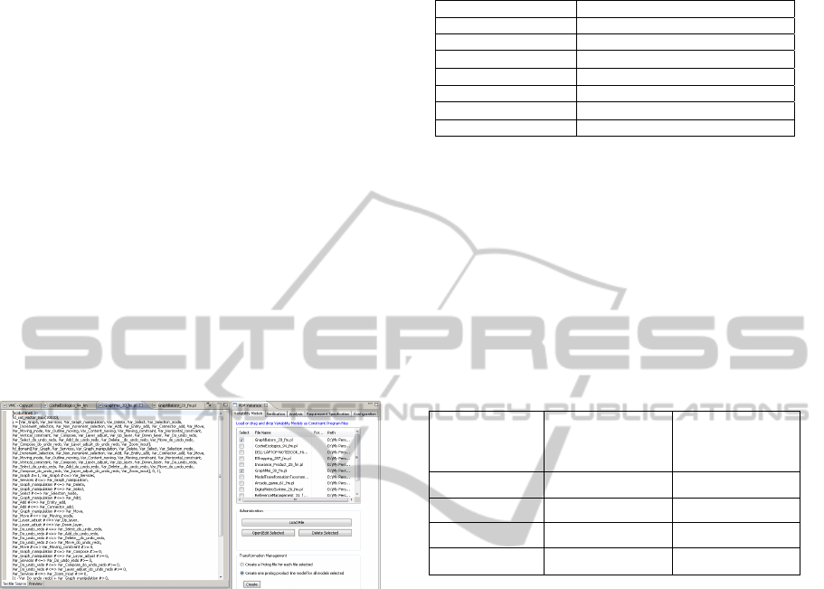
can be passed dynamically to the solver. A snapshot
of the VariaMos interface to translate FMs into CPs
is presented in Figure 3.
Figure 3: Graphical user interface to transform FMs into
constraint programs.
4.2 Scalability
Both transformation strategies were tested in a
laptop computer with Windows vista 32 bits and
with the following characteristics: processor AMD
Turion(tm) X2 Dual-Core Mobile RM-74 of 2,20
MHz and 4,00 GB of RAM.
4.2.1 Transformation using the Navigation
API Strategy
Table 1 shows the average results of our experiment.
These results show that our transformation rules can
be executed in a fast and interactive way by using a
well known API to navigate on FMs.
Table 1: Average time to transform FMs into CPs using
SPLOT.
Number of features Time to transform FMs into CPs
<40 < 1sec
40 to 100 1 sec
101 to 500 1,5 sec
1000 2 sec
2000 3,5 sec
5000 16 sec
10000 70 sec
4.2.2 Transformation using the Engine
Transformation Strategy
Table 2 reports the average time of our experiment.
These figures show that, even for the largest
industrial models considered, our proposal is
scalable and interactive for an engineer in a normal
work environment (no need of additional hardware
or software resources)
Table 2: Average time to transform FMs into CPs using
ATL engine.
Number of
features
Time to transform
FMs into XMI CPs
Time to transform
XMI CPs into
Text CPs
<50 <1 sec < 1sec
50 to 100 3sec <1 sec
101 to 150 5sec 1sec
152 to 180 6,5 sec 1 sec
4.3 Usability
Once the 48 FMS transformed into Benavides et
al.’s (2005), (2005b) and our CP representations, we
executed a series of reasoning operations on these
models. These operations were executed in our
VariaMos tool. The results show an average
reduction of 45% in the execution time of derivation
(e.g., find a product that satisfies given configuration
requirements), verification (e.g., find dead features
and void FMs) and analysis operations (e.g., find the
number of products). Figure 4 shows a time
comparison needed to get a product from a FM
transformed to a CP using both proposals. In Figure
4, we use a log scale to distribute the number of
features (X axis) in order to avoid overlapping of
results on models from 10 to 100 features. This
figure indicates that for the same study conditions
there our transformation rules seem to have a better
performance.
TRANSFORMING ATTRIBUTE AND CLONE-ENABLED FEATURE MODELS INTO CONSTRAINT PROGRAMS
OVER FINITE DOMAINS
195
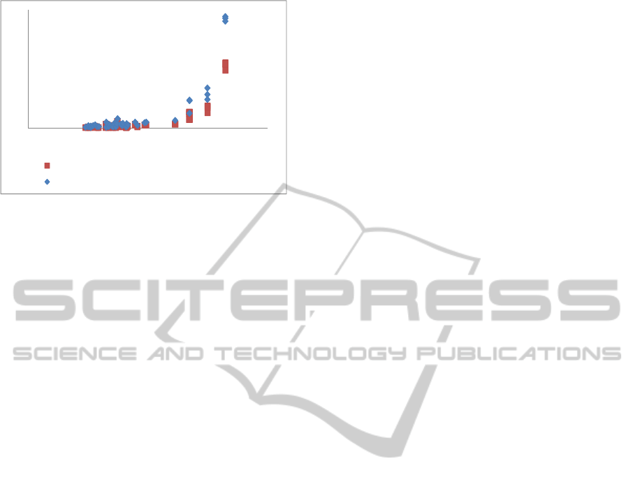
Figure 4: Time (in milliseconds) needed to obtain a
product from a FM. 48 FMs up to 2000 features,
transformed to CP formulas using existing rules and ours.
Finally our approach was also compared to
Karataş’s one (Karataş et al., 2010). Of course, to
perform this comparison, we had to correct the error
we identified in Karataş’ algorithm in order to
preserve the semantic of FMs. This change was
necessary to ensure that both representations were
totally equivalent, by representing the same products
from each FM. Each one of the 12 FMs transformed
in both representations was analyzed using
VariaMos tool. As result of our experiment we have
a benefit of average 58% in the execution time of
each configuration operation –see section 2.3. This
gain is due to the fact that in our representation
algorithm we avoid the combinatorial explosion on
group cardinalities, exclusive relationships and
additional constraints, by using arithmetic
operations. For instance, to constrain the use of only
one feature, among A, B and C in a product, we use
the expression A+B+C=1 instead of: (¬A˄¬B˄C)
∨ (¬A˄B˄¬C) ∨ (A˄¬B˄¬C). And, in the kind
of solver we are using, a CP over integer domain
solver, the first formula is executed faster than the
second one.
4.4 Correctness
The approach that we present in this paper was
compared with the transformation algorithm of
Benavides et al. (2005b). We tested the correctness
of our approach by means of two experiments. The
first one consists in comparing the number of
products that could be derived from our collection of
FMs represented with Benavides’ rules and the rules
presented in this paper. In both cases, the number of
products was equal. The second one consisted in
taking 3 models randomly, manually derive all the
possible products from the FM, then compare these
results with the results obtained using VariaMos. For
practical reasons, we only considered models with
less than 50 features from our initial sample. It is
worth noting that in our comparison we checked, by
manual inspection, that not only the numbers of
products, but also the products themselves, were the
same. These results allow us to conclude that our CP
representation of FMs preserves the semantic of
models. It should be noticed that in our approach,
the structure of FMs is not preserved because it is
not necessary for the 11 reasoning operations that
we execute on FMs (better explained in section 2.3).
Nevertheless, we consider study the impact of FMs’
structure on other kind of eventual reasoning
operations and if some exist we encourage in future
works to represent FMs preserving also their
structure.
5 RELATED WORKS AND
DISCUSSION
Benavides et al. (2005b) present an algorithm to
transform a FODA model into a CP. They suggest
considering four aspects during the mapping a feature
model into a constraint program: (i) the features make
up the set of variables; (ii)
the domain of each
variable is the same: {true, false}; (iii) extra–
functional features are expressed as constraints; and
(iv) every relation of the feature model becomes a
constraint among its features. Benavides (Benavides,
2007) extended their previous work to reason about
constraints specified on feature attributes. Constraints
such as F1.A = F2.B + F3.C can be specified
to express that in any configuration, the value of
attribute A associated with feature F1 should be equal
to B+C where B and C are attributes respectively
associated to F2 and F3. This allows to reason on
extra functional features as defined by Czarnecki et
al. (2005), i.e. relations between one or more
attributes of one or different features. Item (ii) shows
that Benavides’ proposal is a Boolean-based
approach, which limits the use of Integer constraints
(i.e., cardinalities [min..max], where min and
max are integer values and not only limited to 0 or 1).
In addition, their work is limited to FODA-like
models and not pretend to analyse a systems
represented through several model views. Thanks to
our approach it is possible to integrate different views
of the PL in a global model and then analyse it
because in CP, constraints representing different
views can be integrated without a specific order and
the domain of variables is considered as
0
50
100
150
200
250
300
350
400
1 10 100 1000 10000
Time to have a product with our transformation rules
Time to have a product with Benavides' tranformation rules
log
N°features
time
(ms)
ENASE 2011 - 6th International Conference on Evaluation of Novel Software Approaches to Software Engineering
196

supplementary constraints. Views integration and
analysis are out of scope of this paper.
Van Deursen and Klint (2002) proposes to reason
on feature models by translating them into a logic
program using predicates such as all( ), one-
of( ), or more-of(), that respectively specify
mandatory, mutually exclusive, and alternative
features. For instance constraints: F1 = all
(F2, F3, F4), F4 = one-of (F5, F6)
specify that if F1 is included in a configuration, then
F2, F3, and F4, and therefore either F5 or F6
should be included too. The use of CP to reason
about feature model was extended by Batory [2],
who proposes an approach to transform a feature
model into propositional formula using the ∧, ∨, ¬,
⇒ and ⇔ operations of propositional logic. This
enables for example constraints of the form F ⇒ A ∨
B ∨ C meaning that feature F needs features A or B
or C, or any combination thereof. As in (Van
Deursen and Klint, 2002), in these constraints,
features are Boolean variables (either they are
included or not in a configuration). Thus, our
approach not also deals with Boolean constraints but
also Arithmetic constraints, Symbolic constraints
and Reified constraints over finite-domain variables.
Integer CP allows us to execute requirements as:
“the value of attribute F1.A should always be equal
to F2.B + F3.C” to control the value of integer
feature attributes, as proposed by (Benavides, 2007).
As well as to control the number of occurrences of a
feature, as for instance in the constraint “a product
should include at least 2 and at most 4 occurrences
of feature F”. Feature cardinalities were proposed
by Czarnecki et al. (2005), but constraint analysis on
feature cardinalities has not yet been tackled to our
knowledge (Benavides et al., 2010), and there is no
tool available so far to support the analysis of
constraints on feature cardinalities and on feature
attributes in an integrated way. Finite domain
constraints can also apply on any ENUM PL
properties, like in the Decision King tool which uses
them to control decision consistency (Dhungana et
al., 2007). CP also enables the specification of
“complex” product requirements (complex
compared to select or not a feature) under the form
of additional constraints specified during the
configuration. For example, our approach supports
the specification of constraints such as “provide me
with all possible configurations in which the value of
feature attributes A1..Ai is in [a..b]”. This is useful
in staged configuration (Djebbi and Salinesi, 2007).
Other new kinds of product-specific constraints such
as: “provide with a configuration in which the
values of all the attributes associated with features
F1..Fn are different from each other”, and “provide
me with all product configurations in which features
F1...Fn are either all included or all excluded” or
“provide me with the features that have not the
chance to be selected (dead features)”. Such
constraints can be used to query the PL model, that
is useful for instance to explore configuration
scenarios, or in a verification activity.
Recent work by Karataş et al. (2010) proposes a
transformation from extended feature models to CP.
This work considers neither the actual semantic of
features’ attributes, as it considers them as sub-
features that can be selected or not, nor the semantic
of cardinality-based feature models as it was
validated by the community (Michel et al., 2011).
Our work goes a step further by testing our
transformation patterns on the most complete set of
feature models publicly available. Additionally, the
transformation patterns used by Karataş considers
only boolean formulas to represent extended feature
models, which reduces the richness of the constraint
programming paradigm, a richness that we believe is
necessary to represent complex feature models and
to support advanced reasoning (e.g. to detect the
optimal product according to a cost criterion).
Besides, we detected an error in their CP
representation regarding optional features. Karataş et
al.’s representation of optional features allows
selection of child features without constraining the
selection of the father feature.
6 CONCLUSIONS AND FUTURE
WORK
In this paper we provide an approach to transform
FMs with attributes and feature cardinalities into
constraint programs. To our knowledge, it is the first
time that a proved representation of these kinds of
models is presented. Once our 60 FMs represented
as constraint programs, we applied on them our
collection of 11 reasoning operations, completely
automated in our tool VariaMos and the CP solver
GNU-Prolog (Diaz and Codognet, 2001). We use
GNU-Prolog to reason on FMs, but other solver can
be used as another alternative. Even if GNU-Prolog
is not the best solver to implement some reasoning
operations on very large models (e.g. to calculate the
number of products or to list all the products of a
FM), it performed well and showed an excellent tool
for other kind of reasoning (e.g. determining if a FM
is void or not, to find dead features, false optional
TRANSFORMING ATTRIBUTE AND CLONE-ENABLED FEATURE MODELS INTO CONSTRAINT PROGRAMS
OVER FINITE DOMAINS
197

features, non attainable domains of a variable or in
the case of configuration with and without extra-
requirements).
As future work, we are considering, in one hand, to
work on other type of reasoning operations on
product line models. And on the other hand, we
propose an experimental design to evaluate the
performance, memory consumption and precision of
these operation when we implement then in different
solvers (SAT, CSP, CLP, BDD, ADD, etc.).
Additionally, we propose to work in multidirectional
transformation, because our up-to date work only
considers unidirectional transformations.
REFERENCES
Batory, D. S., 2005. Feature models, grammars, and
propositional formulae. In: 9th International Software
Product Lines Conference, pp. 7–20. Springer.
Benavides, D., 2007. On the Automated Analysis of
Software Product Lines Using Feature Models. A
Framework for Developing Automated Tool Support.
University of Seville, Spain, PhD Thesis.
Benavides, D., Ruiz-Cortés, A., Trinidad, P., 2005. Using
constraint programming to reason on feature models.
In: The Seventeenth International Conference on
Software Engineering and Knowledge Engineering,
SEKE 2005, pp. 677–682.
Benavides D., Segura S., Ruiz-Cortés A., 2010.
Automated Analysis of Feature Models 20 Years
Later: A Literature Review. Information Systems.
Elsevier.
Benavides, D., Trinidad, P., Ruiz-Cortés, A, 2005.
Automated Reasoning on Feature Models. In: Pastor,
Ó., Falcão e Cunha, J. (eds.) CAiSE 2005. LNCS, vol.
3520, pp. 491–503. Springer, Heidelberg.
Bessiere, Ch., 2006. Constraint propagation. In Francesca
Rossi, Peter van Beek, and Toby Walsh, editors,
Handbook of Constraint Programming, pages 29–83.
Elsevier.
Czarnecki, K., Helsen, S., Eisenecker, U., 2005.
Formalizing cardinality-based feature models and their
specialization. Software Process: Improvement and
Practice, 10(1):7– 29.
Dhungana, D., Heymans, P., and Rabiser, R., 2010. A
Formal Semantics for Decision-oriented Variability
Modeling with DOPLER, Proc. of the 4th
International Workshop on Variability Modelling of
Software-intensive Systems (VaMoS 2010), Linz,
Austria, ICB-Research Report No. 37, University of
Duisburg Essen, pp. 29-35.
Dhungana, D., Gruenbacher, P., Rabiser, R., 2007.
DecisionKing: A Flexible and Extensible Tool for
Integrated Variability Modeling. In: 1rst Int.
Workshop VaMoS, pp120-128, Ireland.
Diaz, D., Codognet, P., 2001. Design and Implementation
of the GNU Prolog System. Journal of Functional and
Logic Programming. http://www.gprolog.org.
Djebbi, O., Salinesi, C., 2007. RED-PL, a Method for
Deriving Product Requirements from a Product Line
Requirements Model. In: CAISE’07, Norway.
Gurp, J. v., Bosch, J., Svahnberg, M., 2001. On the Notion
of Variability in Software Product Lines. In
Proceedings of the Working IEEE/IFIP Conference on
Software Architecture (WICSA).
Halmans, G., Pohl, K., 2003. Communicating the
variability of a software-product family to customers.
Softw Syst Model. 2: 15–36 / Digital Object Identifier
(DOI) 10.1007/s10270-003-0019-9.
Kang, K., Cohen, S., Hess, J., Novak, W., Peterson, S.,
1990. Feature-Oriented Domain Analysis (FODA)
Feasibility Study. Technical Report CMU/SEI-90-TR-
21, SEI, Carnegie Mellon University.
Kang, K., Lee, K., Lee, J., 2002. FOPLE - Feature
Oriented Product Line Software Engineering:
Principles and Guidelines. Pohang University of
Science and Technology.
Karataş A. S, Oğuztüzün H., Do
ğru A., 2010. Mapping
Extended Feature Models to Constraint Logic
Programming over Finite Domains. SPLC, Korea.
Mazo, R., 2010. VariaMos Eclipse plug-in: https://
sites.google.com/site/raulmazo/
Mazo, R., Grünbacher, P., Heider, W., Rabiser, R.,
Salinesi, C., Diaz, D., 2011. Using Constraint
Programming to Verify DOPLER Variability Models.
5th ACM International Workshop on Variability
Modelling of Software-intensive Systems (VaMos'11),
Namur-Belgium.
Mazo R., Lopez-Herrejon R., Salinesi C., Diaz D., Egyed
A., 2011. A Constraint Programming Approach for
Checking Conformance in Feature Models. In 35th
IEEE Annual International Computer Software and
Applications Conference (Compsac'11). Munich-
Germany.
Mendonça, M., Branco, M., Cowan, D., 2009. S.P.L.O.T.:
software product lines online tools. In OOPSLA
Companion. ACM, http://www.splot-research.org.
Mendonça, M., Wasowski, A., Czarnecki, K., 2009. SAT–
based analysis of feature models is easy. In
Proceedings of the Sofware Product Line Conference.
Michel, R., Classen, A., Hubaux, A., Boucher, Q., 2011. A
Formal Semantics for Feature Cardinalities in Feature
Diagrams. 5th International Workshop on Variability
Modelling of Software-intensive Systems (VaMos'11),
Namur-Belgium.
Nuseibeh, B. Easterbrook, S., 2000. Requirements
Engineering: A Roadmap, The Future of Software
Engineering, 22nd Int. Conf. on Soft. Eng., 37-46,
ACM, Washington.
Salinesi, C., Mazo, R., Diaz, D., 2010. Criteria for the
verification of feature models, In 28th INFORSID
Conference, Marseille, France.
Salinesi, C., Mazo, R., Diaz, D., Djebbi, O., 2010b.
Solving Integer Constraint in Reuse Based
Requirements Engineering. 18th IEEE International
Conference on Requirements Engineering (RE'10).
Sydney, Australia.
ENASE 2011 - 6th International Conference on Evaluation of Novel Software Approaches to Software Engineering
198

Salinesi C., Mazo R., Djebbi O., Diaz D., Lora-Michiels
A, 2011. Constraints: the Core of Product Line
Engineering. Fifth IEEE International Conference on
Research Challenges in Information Science (IEEE
RCIS), Guadeloupe-French West Indies, France.
Schobbens, P. Heymans, P. Trigaux, J. Bontemps, Y.,
2007. Generic semantics of feature diagrams, Journal
of Computer Networks, Vol 51, Number 2.
Schulte, Ch., Stuckey., P. J., 2008. Efficient constraint
propagation engines. ACM Trans. Program. Lang.
Syst., 31(1).
Streitferdt, D., 2004. FORE Family-Oriented
Requirements Engineering, PhD Thesis, Technical
University Ilmenau.
Van Hentenryck, P., 1989. Constraint Satisfaction in
Logic Programming. The MIT Press.
Van Deursen, A., Klint, P., 2002. Domain–specific
language design requires feature descriptions. Journal
of Computing and Information Technology, Vol. 10,
No. 1.
Ziadi, T., Helouet, L., Jezequel, J.-M., 2003. Towards a
UML Profile for Software Product Lines. In: Software
Product- Family Engineering, 5th International
Workshop, pages 129– 139. Springer.
TRANSFORMING ATTRIBUTE AND CLONE-ENABLED FEATURE MODELS INTO CONSTRAINT PROGRAMS
OVER FINITE DOMAINS
199
