
MULTIPLE MOBILE SYNCHRONISED SINKS (MMSS) FOR
ENERGY EFFICIENCY AND LIFETIME MAXIMIZATION
IN WIRELESS SENSOR NETWORKS
H. Sivasankari, Vallabh M., Shaila K. and K. R. Venugopal
University Visvesvaraya College of Engineering, Bangalore University, Bangalore 560 001, India
L. M. Patnaik
Vice Chancellor, Defence Institute of Advanced Technology (Deemed University), Pune, India
Keywords:
Energy efficiency, Lifetime maximization, Multiple mobile sink, Sojourn time and wireless sensor networks.
Abstract:
Wireless Sensor Networks(WSNs) consist of battery operated sensor nodes. Improving the lifetime of sensor
network is a critical issue. Nodes closer to the sink node drains energy faster due to large data transmission
towards a sink node. This problem is resolved through mobility of the sink node. The Mobile sink moves
to particular positions in predetermined order to collect data from the sensor nodes. There is considerable
delay in the case of single mobile sink. In this paper we have used the concept of multiple mobile sinks to
collect data in different zones which in turn coordinate to consolidate the data and complete the processing
of data received from all the sensor nodes. A distributed algorithm synchronizing all the mobile sinks are
used to reduce the delay in consolidation of data and reducing the overall energy consumption. The twin gain
increases the lifetime of the Wireless Sensor Network. Simulation results using Multiple Mobile Synchronized
Sinks clearly shows that there is an increase of 28% and 56% in the lifetime of the Wireless Sensor Networks
in comparison with Single Mobile Sink and Static Sink respectively.
1 INTRODUCTION
Wireless Sensor Network (WSNs) uses battery op-
erated wireless micro-sensor nodes to collect the in-
formation from a geographical field and transmits in
multihops to the sink. Hundreds or thousands of this
micro-sensors are deployed to watch the environment
and collects the data about it. These sensor batteries
are impractical to replace or recharge and hence en-
ergy of the sensor nodes are to be saved to increase
the lifetime of the Network. The operational lifetime
of a sensor node is in terms of weeks or months. Sen-
sor node spends energy for each process like sensing,
transmitting and receiving data. Hence, energy is an
important criteria in Wireless Sensor Networks.
WSNs have considerable technical challenges in
data processing and communication to deal with dy-
namically changing Energy, Bandwidth, Delay, Sens-
ing and Processing power. The vital issue in WSNs
is to maximize the network operational life. In order
to achieve this, it is necessary to minimize the energy
utilization of every sensor node. Energy can be conse-
rved by efficient routing and data aggregation. An-
other important issue in WSNs is security when it op-
erates in a hostile environment and needs to be pro-
tected against intruders.
For the small networks, source sensors can di-
rectly transmits the data to the sink node. For a larger
network, multihop communication is needed to reach
the static sink. For real time applications, the sensi-
tive data should reach the sink node without any de-
lay. There are many methods to reduce the distance
between the source and the sink. First method is to
move the sink node over the entire network to collect
the data, the second method is to have multiple static
sinks at different locations and third method is to in-
crease the number of mobile sinks. Thus the distance
between the source and sink is reduced.
When an event occurs, immediately the sensor
node communicates the information to the sink node.
Neighbor nodes of the sink node depletes energy
faster due to the large and continuous data forward-
ing towards the sink. Thus, lifetime of the sensor
network is reduced even though non-neighbor nodes
76
Sivasankari H., M. V., K. S., R. Venugopal K. and M. Patnaik L..
MULTIPLE MOBILE SYNCHRONISED SINKS (MMSS) FOR ENERGY EFFICIENCY AND LIFETIME MAXIMIZATION IN WIRELESS SENSOR
NETWORKS.
DOI: 10.5220/0003499500760085
In Proceedings of the 13th International Conference on Enterprise Information Systems (ICEIS-2011), pages 76-85
ISBN: 978-989-8425-56-0
Copyright
c
2011 SCITEPRESS (Science and Technology Publications, Lda.)

haveenough energy for communication. To overcome
this problem Gatzianas et al., (Gatzianas and Geor-
giadis, 2008) have considered the use of single mo-
bile sink. The mobile sink collects the information
from the sensor nodes during its round trip time i.e.,
time during which mobile sink visits entire network
in predetermined positions.
Motivation. In static sink sensor network, nodes
closer to the sink depletes their energy fast, though
other nodes in a network have enough amount of
energy for communication. The single mobile sink
keeps moving to predetermined positions and stays
for a specific period of time to collect the data. The
sensitive data moving from the source sensors may
loose their importance due to the nonavailability of
the single mobile sink. This is due to the delay in
the arrival of the single mobile sink to that position.
This problem is addressed in this paper by implement-
ing distributed algorithm with multiple mobile sinks
and thus sensitive information reaches the sink with-
out delay.
Contribution. The main contribution of this paper
is the development of an efficient distributed algo-
rithm using Multiple Mobile Synchronized Sinks of-
fering an alternative to the single mobile sink. A dis-
tributed algorithm for computing the maximum life-
time of a wireless sensor network, which routes data
to the nearest mobile sink by imposing flow con-
servation to all positions with respect to sinks. An
interference-free sensor network with a multiple mo-
bile synchronized sinks reduces delay, uses less Band-
width, consumes lower energy and increases the life-
time of the WSNs.
Organization. The rest of the paper is organized as
follows: Related work and Background work are dis-
cussed in Section 2 and Section 3 respectively. Sys-
tem Model and Network Architecture are explained
in Section 4. Problem Definition and Mathematical
Model is formulated in Section 5. Algorithm is de-
veloped in Section 6. Simulation and Performance
parameters are analyzed in section 7. Conclusions are
presented in Section 8.
2 RELATED WORK
Gatzians et al.,(Gatzianas and Georgiadis, 2008) ad-
dressed the maximization of lifetime of a mobile sink
WSNs in-terms of energy constraint. A distributed
Synchronous ε -relaxation algorithm based on the
subgradient method is presented to minimize the re-
quired time to route data from other nodes of the net-
work to a mobile sink. The system is restricted to
semi-deterministic settings resulting in considerable
delay.
Michail et al.,(Michail and Ephremides, 2003)
discussed the routing connection-oriented traffic in
wireless sensor networks with energy efficiency. Min-
imization of data transmission cost with limited band-
width resources have been considered. Real-time con-
straints in the system and the restriction of nodes to
the boundary of location leads to long routing paths
between end to end nodes.
Xiao et al.,(Xiao et al., 2004) focused on link
based optimal routing in wireless data networks. They
have exploited a Simultaneous Routing Resource Al-
location (SRRA) problem and capacitated multicom-
modity flow model to describe the data flows in the
WSN. Joint link scheduling, routing and power allo-
cation are not emphasized in this work.
Chang et al.,(Chang and Tassiulas, 2000) consid-
ered flow augmentation, flow redirection algorithm to
balance the energy among the nodes in proportion to
their reserve energy. The robustness of Shortest path
routing to maximize the lifetime of a network is not
discussed in this work.
Madan et al.,(Madan and Lall, 2006) formulated
a distributed algorithm to compute an optimal routing
scheme. The algorithm derived the concept of convex
quadratic optimization & time constraint to maximize
the lifetime of network. They have not considered
asynchronous sub-gradient algorithm.
Ritesh et al.,(Madan et al., 2005) discussed the
mixed integer convex program to maximize the life-
time of network. Non linear class of interference
free Time Division Multiple Access for load balanc-
ing, Multihop routing frequency reuse & interference
mitigation are utilized to increase lifetime of net-
work. The work is restricted for non-distributed low
topologised model with lower bound. Shashidhar et
al.,(Gandham et al., 2003)proposed a flow based rout-
ing protocol to minimize the energy consumption in
the sensors of WSNs.
Weiwang et al., (Weiwang and Chua, 2005) have
used mobile relays to prolong the lifetime of Wireless
Sensor Networks. The lifetime of the dense sensor
network with mobile sink and mobile relays are al-
most same as that of mobile sink.
Branislav et al.,(Kusy et al., 2009) have developed
an algorithm for data delivery in mobile sensor net-
works. Mobility patterns in the network, enables the
algorithm to maintain an uninterrupted data stream.
Scalability and communication cost are not consid-
ered.
Huang Zhi et al., (Zhi et al., 2010) have developed
routing strategies for Dynamic WSN with single sink
and multiple sinks. DWSN with single static sink is
MULTIPLE MOBILE SYNCHRONISED SINKS (MMSS) FOR ENERGY EFFICIENCY AND
LIFETIMEMAXIMIZATION INWIRELESS SENSOR NETWORKS
77

more reliable than the multiple static sinks. Frequent
changes of routing table consumes more energy and
the lifetime of Dynamic WSN is reduced with long
latency and weak reliability.
Getsy et al.,(Getsy et al., 2010) proposed cluster
based routing protocol for Mobile WSN (MWSN).
Bayes rule is used in selection of cluster head with
highest energy, least mobility and best transmission
range. It is not fault tolerant.
3 BACKGROUND
Nodes in a Wireless Sensor Network produces infor-
mation at a deterministic rate. Sensor Nodes nearer
to the static sink, drains energy soon because of large
data transmission to the sink node. To increase the
lifetime of the sensor network Luo et al.,(Luo et al.,
2005) considered a single mobile sink. Each node
drains energy as the mobile sink moves to close to a
position of occurrence of an event, spends a specified
amount of time to collect the data from the sensors
around the location of occurrence of the event.
The following conditions are assumed to give fea-
sible solutions to the outgoing links of node to max-
imize the lifetime. The total expended power should
not exceed the initial reserve energy. A peak power
transmission constraints are imposed in all the loca-
tion of sink and time intervals. A mobile sink can re-
side in a particular location for nonzero sojourn time
and when sojourn time becomes zero, it moves to the
next location.
In a distributed algorithm each node must store
the following information., (i) Sink is distinguished
from other nodes by unique node tag identifier,(ii)
The maximum rate of information, energy and in-
stantaneous power for each node, (iii) group of vari-
ables representing the flow and flow conservation cost
which are used in minimum cost flow algorithm. (iv)
the outgoing and incoming edges are doubly linked
list, (v) a maximum array length to store parent and
children of the node, (vi) variables independent of
Network size.
4 SYSTEM MODEL AND
NETWORK ARCHITECTURE
4.1 Definitions
Mobile Sink. One mobile sink moves to the pre-
determined positions collecting data from all the
neighboring nodes.
Synchronized Sinks. Synchronization of multiple
mobile sink is achieved through the common no-
tion of time.
Multiple Mobile Sinks. More than one mobile sink
moves to the predetermined positions collecting
data from all the neighboring nodes.
Sojourn Time. The duration of time during which
active mobile sink resides in a particular position.
Network Alive. The Network is alive until the sen-
sor can transfer all generated traffic to the nearest
sink by satisfying the energy/power and flow con-
servation constraints.
Energy Consumption. The amount of energy spent
by each node in a sensor network for sensing,
sending, receiving and processing data.
Lifetime of a Network. The period of time until the
first node runs out of energy.
Delay. Time taken by the data to reach the mobile
sink node from the source sensor node.
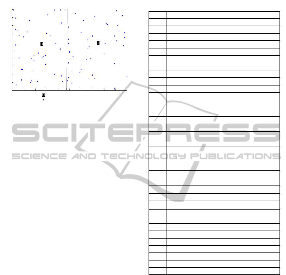
4.2 Network Architecture
The Multiple Mobile Synchronized Sink WSNs con-
sists of two types of nodes, (i) Static ordinary sensor
nodes which can only capture and transmit data, (ii)
Mobile sink nodes that move to predetermined po-
sitions to collect data from the static Sensor nodes.
Multiple mobile sink nodes can coordinate to con-
solidate data collected from the static sensor nodes.
The Wireless Sensor Network is divided into a num-
ber of zones as shown in Figure 1. The movement
of the mobile sink is restricted to its zone. This tech-
nique increases the collection of data from ordinary
sensor nodes reducing the consumption of energy and
delay. Both these features helps in increasing the life-
time of WSNs. When one of the sink fails, the zones
are merged. The network still continues to function
though at a reduced efficiency, there is increase in
delay and is called graceful degradation. The em-
ployment of multiple mobile sink increases reliabil-
ity and does not allow the WSNs to collapse even
with the failure of some Mobile sinks. The multiple
mobile sinks are in continuous communication syn-
chronously and thereby any failure in the sinks will
be immediately detected and can be rectified.
4.3 Network Model
Consider a Wireless Sensor Network consisting of
battery operated static nodes, which are randomly de-
ployed over a given geographical area. The system
model for the mobile sinks x
m
, moves to fixed position
ICEIS 2011 - 13th International Conference on Enterprise Information Systems
78
0 10 20 30 40 50 60 70 80 90 100
0
10
20
30
40
50
60
70
80
90
100
1
2
3
4
5
6
7
8
9
10
11
12
13
14
15
16
17
18
19
20
21
22
23
24
25
26
27
28
29
30
31
32
33
34
35
36
37
38
39
40
41
42
43
44
45
46
47
48
49
50
51
52
53
54
55
56
57
58
59
60
61
63
64
65
66
67
68
69
70
71
72
73
74
75
76
77
78
79
80
62
Ordinary Node
Mobile Sink Node
Figure 1: Basic Multiple Mobile Sink Wireless Sensor Net-
work Architecture.
x
p
m
to avoid early energydissipation of neighbor nodes
of the sink (i.e., as in static sensor network)(Luo,
2006). Each node sensor i = 1,.......,n ∈ V produces
a fixed amount of information at rate of I
i
≥ 0. It is
assumed that all links between the nodes are bidirec-
tional. The notations used in this paper are defined in
Table 1.
The movement of the sinks to different positions
creates a subgraph G(V,L). All nodes i ∈ V except for
the sink are equipped with a non-renewable amount
of energy E
i
> 0. The energy of the sensor is gradu-
ally depleted as the nodes participate in routing. Once
a node’s energy is drained, the node can no longer
transmit which leads to network failure.
5 PROBLEM DEFINITION AND
MATHEMATICAL MODEL
5.1 Problem Definition
Given a set of Wireless Sensor Nodes i ∈ V, where
i = 1,......, n and set of mobile sinks, t
p
x
m
the sojourn
time of the m
th
sink at position p, t
p,k
x
m
for a set of
iterations where k = 1, .....,K. The objectives are
1. To decrease energy consumption and increase the
lifetime of the Wireless Sensor Network.
2. To find optimal routing, maintain synchronization
between the mobile sinks, to improve sojourntime
and increase the survival time of the network (T).
Where
max T =
p
∑
1
K
∑
k=1
x
p,k
m
(1)
Table 1: Notations.
G Undirected Graph.
V Set of sensor nodes.
L Edge set or link set.
S
i
Source node i, i = 1,...,n.
x
m
m
th
mobile sink.
i Single sensor node, i ∈ V.
S
p
i
set of outgoing neighbors of node i
at sink at position p.
I
i
Information generated at the node i.
x
p
m
p
th
position of the mobile sink x
m
, p ∈ P.
P set of mobile sinks positions.
R
p,k
ij
Data transmission rate from node i to j
while sink stays at position p for k
th
iteration.
R
p
ij
Data transmission rate from node i to j
while sink stays at position p.
t
p,k
x
m
Time for k
th
iteration of m
th
mobile sink
at position p.
e
p,k
ij
Power needed for data transmission from
node i to j while sink stays at position p
for k
th
iteration.
e
p
ij
Power needed for data transmission from
node i to j while sink stays at position p.
t
p
x
m
Sojourn time of the m
th
sink at position p.
E
i
Initial Energy of the node.
G
′
Sub graph G
′
⊂ G.
e
t
Power needed for transmitting one bit of
data.
e
r
Power needed for receiving one bit of data.
k
r
k bits of data is received.
k
t
k bits of data is transmitted.
α transmission factor.
β reception factor.
ε
i
power constraint
d
ij
distance between node i and j
and can be further reduced to a equivalent form of
max T =
p
∑
1
t
p
x
m
(2)
From Equation 2, we can calculate the maximum
lifetime of each mobile sink at different positions.
Assumptions
1. Sensor nodes are stationary, but the sinks change
their positions from time to time with negligible
traveling time between two positions. The posi-
tions of the sinks can be chosen within a finite set
of x
p
m
∈ P.
MULTIPLE MOBILE SYNCHRONISED SINKS (MMSS) FOR ENERGY EFFICIENCY AND
LIFETIMEMAXIMIZATION INWIRELESS SENSOR NETWORKS
79

2. A mobile sink has long range of communication
that facilitates to transmit data.
3. Each sensor i ∈ V produces information at fixed
deterministic rate I
i
≥ 0, which is routed in multi-
hops to one of the mobile sinks x
m
.
5.2 Mathematical Model
For receiving k
r
bits/sec, the power consumption at
sensor node is e
r
= k
r
β. where, β is reception factor
indicating the energy consumption per bit. The power
needed for transmitting k
t
bits/sec is e
t
= k
t
αd
ij
.
where, α is transmission factor indicating the energy
consumption per bit and d
ij
is the distance between
transmitting and receiving node. Therefore, total en-
ergy consumption at a node per time unit is
e
r
+ e
t
= k
r
β+ k
t
αd
ij
≈ e(k
r
+ k
t
) (3)
where, e = β ≈ α d
ij
, because energy consumed to
transmit a bit is approximately equal to the energy
consumed for receiving a bit.
From the above discussions, the energy consump-
tion at a sensor node i when the sink sojourn at posi-
tion p is computed as
e
p
ij
= e(
∑
j∈S
p
i
R
p
ij
+
∑
j:i∈S
p
j
R
p
ji
) (4)
where, e
p
ij
represents the total power needed for data
transmission from node i to j while sink stays at
position p. The energy is calculated through data
transmission rate from node i to j and j to i vice
versa with respect to the sink’s position.
p
∑
1
∑
j ∈ S
p
i
R
p
ij
e
p
ij
t
p
x
m
≤ E
i
∀ i ∈ N (5)
∑
j ∈ S
p
i
R
p
ij
e
p
ij
≤ ε
i
, ∀ i ∈ N, ∀ p ∈ P (6)
∑
j∈S
p
i
R
p
ij
= I
i
+
∑
j:i∈S
p
i
R
p
ji
(7)
The sink is moving through robots. The entire geo-
graphical deploymentarea has dividedinto two zones.
In each zone sinks moves to the predefined positions.
The mobile sink moves to different positions to col-
lect the data from the source node. When an event
occurs, the sensor senses the data and it forwards the
data to the nearest mobile sink positions. If sink is
not available in that position then sensors forwards the
data to the next available position of the sink. We re-
duce the Response Time (RT) by introducing the mul-
tiple mobile sinks. The Response Time is computed
as,
RT = RT
end
− RT
start
(8)
RT
start
is the time during which the packet started.
RT
end
is the time during which the packet reached the
sink.
Equation 4 represents the total amount of energy
spent at node i and j that depends on the traffic rate
on node i and j. Equation 5 and 6 explains the energy
constraints for communication i.e., energy required
for transmitting and receiving data, must not exceed
the residual energy of a node. Equation 7 gives the
data transmission rate on link i, j i.e., the sum of ac-
tual sensed information and traffic rate in the link.
6 ALGORITHM
6.1 MMSS Distribution Algorithm
The Multiple Mobile Synchronized Sink algorithm
comprises of two algorithms: MMSS Routing Algo-
rithm and MMSS Iteration Algorithm. In Table 2 the
MMSS Distribution Algorithm begins with the selec-
tion of multiple mobile sinks. Each sink moves to a
predefined position for a specified period of time to
collect data from each zone. The neighbors of a ac-
tive sinks are identified by sending the hello packets
from all the sensor nodes to the nearest active sink.
MMSS algorithm runs for various iterations for dif-
ferent sinks and positions.
MMSS Routing Algorithm selects a minimum
distance routing to reduce the energy consumption in
the network. When a sensor node has data to forward,
it checks for the active sink position and then forwards
the data. If the data transmission time exceeds the
sink’s sojourn time then forwards the data to the next
nearest active position of the mobile sink.
The data collection during the sojourn time of the
mobile sink is referred as iterations (i.e., number of
successive transmission). Number of iterations for a
particular sink is computed by summing the number
of successive transmission during its round trip. The
amount of energy dissipated by each node for trans-
mission and reception of data is calculated. If residual
energy is equal to zero then network fails. Other-
wise, the algorithm runs until one of the node’s en-
ergy drains to zero in the network. Failure in the sink
is detected and repaired as the sinks are synchronized.
7 IMPLEMENTATION AND
PERFORMANCE ANALYSIS
In the setup of MATLAB simulation, a 100m x 100m
region was considered with three sets of network
ICEIS 2011 - 13th International Conference on Enterprise Information Systems
80
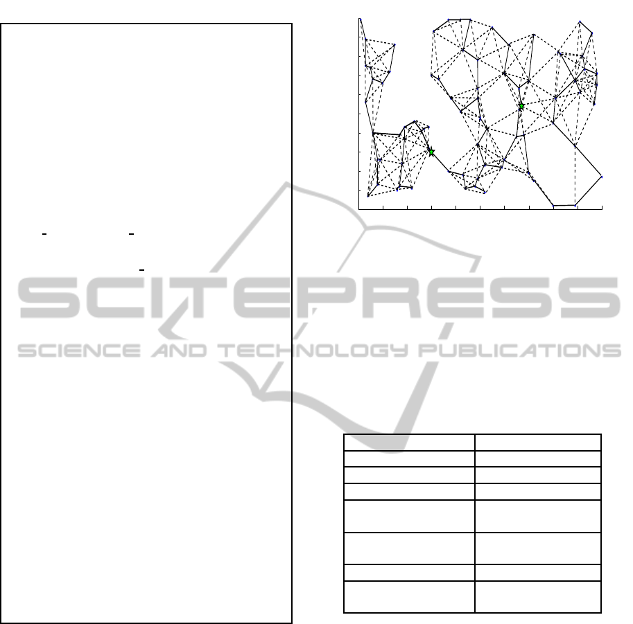
Table 2: MMSS Distribution Algorithm.
The subgraph G
′
∈ G for all k, vectors V,E, P,I,ε
initial iteration k
0
are taken as input to the algorithm
Initialize k = k
0
Select x
m
as the number of mobile sinks and predeter-
mine positions as x
p
m
.
Fix the routing path of each sink x
m
;
set arbitrary time t;
while termination criterion is false do
for p = 0 to |P| − 1 do
Phase 1: MMSS Routing Algorithm
for i = 1 to n− 1 do
for j = i+ 1 to n do
Calculate the distance between all the nodes with
respect to the active position of the sink x
p
m
at time t.
total distance = total distance+ distance ;
endfor
endfor
compute minimum total distance
solve the minimum cost flow for subgraph G
′
determine t
p
x
m
;
if t
p
x
m
≥ transmission time then
Route the data to the nearest active position of the
sink x
m
else Route the data to the next nearest active position
of the sink x
m
endif
Phase 2: MMSS Iterations Algorithm
update t
p
x
m
∀(i, j) ∈ L
update from k to k + 1 for all nodes
endfor
Calculate Energy dissipation as
Energy dissipation = Transmission Power +
Flow Rate;
Calculate Residual energy of the node
E
i
= Residual Energy − Energy dissipation;
if E
i
= 0 then
return;
else
k = k + 1;
endif
if sink x
m
is failed then x
m+1
is made active for that
zone.
endif
endw
topology with 20, 40 and 80 nodes respectively. The
sink was allowed to move over 2, 4 and 8 locations,
which were the same for all zones. In all cases, each
node had an exogenous rate of I
i
= 1. The flow cost of
edge L(i, j) is assumed proportional to d
ij
the physi-
cal distance between the two nodes. Two scenarios
were studied: in the first one, only a power constraint
of E
i
= 100nJ is applied while in the second one, a
power constraint of ε
i
= 10nJ is also imposed. The
simulation parameters are shown in Table 3.
We consider, as nodes increase in a sensor net-
works, the number of mobile sinks also increases. The
Simulation environment deployed with 8x10 i.e., 80
nodes. Each node is identified through node identi-
0 10 20 30 40 50 60 70 80 90 100
0
10
20
30
40
50
60
70
80
90
100
4
58
Figure 2: Complete Route tree for Multiple mobile sink in
100X100 area with 80 nodes.
fier as node 1, node 2, node 3 etc... The simulation
setup is varied for 20, 40, 80 nodes with multiple mo-
bile sinks. Mobile sink moves in 2, 4, 8 locations and
stays for a sojourn time. We observe that, there is a
considerable increase in the lifetime of a multiple mo-
bile sink of Sensor Network in comparison with static
and single mobile sink.
Table 3: Simulation Parameters.
Parameter Type Test values
Number of nodes 100
sink node mote 1
Radio model lossy
Multi channel Radio 433MHz
Transceiver
Sensor type Light, Temperature,
Pressure
Outdoor Range 500ft
Energy consumption 60pJ
per bit
Table 4, Table 5 and Table 6 gives the amount of
energy residues in each node of 8x10 simulation setup
after 914, 1386 and 1646 iterations of Sensor Net-
work with static sink, single mobile sink and multiple
mobile sink respectively. Table 4 shows the residual
energy of nodes for single static sink. In the table
zeroth row and first column represents node 1, the ze-
roth node and second column represent node 2 and
the first row and first column represent node 11 in this
manner nodes 1 to node 80 are identified. The amount
of energy residues in node 1 is 1.378nJ.
Table 4 gives the residual energy of the node for
the network with the static sink. We observe that
nodes 25, 36, 45 and 66 closer to the static sink have
zero energy remaining and the network fails after 914
MULTIPLE MOBILE SYNCHRONISED SINKS (MMSS) FOR ENERGY EFFICIENCY AND
LIFETIMEMAXIMIZATION INWIRELESS SENSOR NETWORKS
81
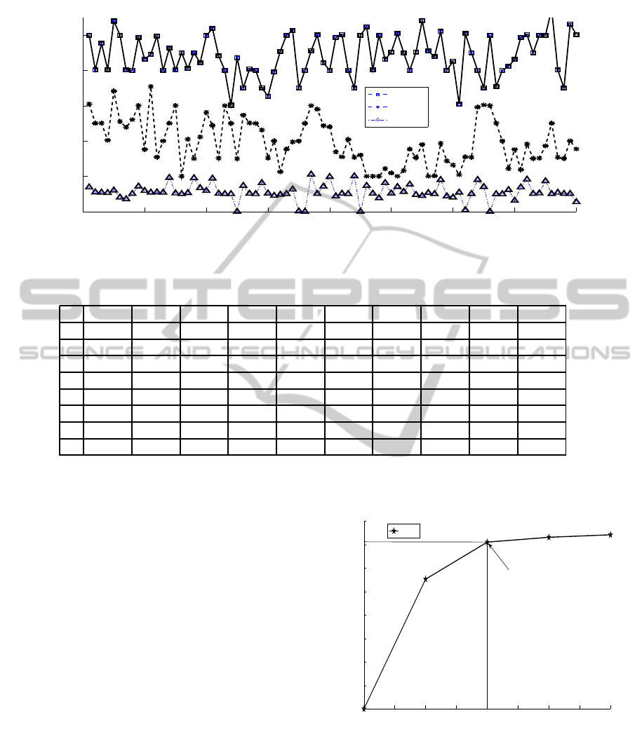
0 10 20 30 40 50 60 70 80
0
2
4
6
8
10
Number of Sensor Nodes
Residual Energy in the sensor node(nJ)
MMSS
MS
SS
Figure 3: Comparison between the MMSS, SMS and SS Networks after 914 iterations.
Table 4: Residual Energy(nJ) in each node of 8x10 static sink WSNs after 914 iterations.
1 2 3 4 5 6 7 8 9 10
0 1.378 1.096 1.085 1.062 1.204 0.805 0.706 1.009 1.430 1.180
1 1.085 1.096 1.08 1.92 1.04 1.001 1.056 1.900 1.340 1.185
2 1.876 1.021 1.002 1.000 0.000 1.467 1.024 1.000 1.623 1.035
3 0.902 0.963 1.001 1.258 0.020 0.000 2.109 1.008 1.424 1.970
4 0.876 1.021 1.002 2.009 0.000 1.467 1.024 0.767 1.623 1.035
5 1.402 1.125 1.535 0.952 0.890 1.060 1.003 1.800 0.873 0.803
6 1.085 0.086 1.007 1.802 1.401 0.000 0.996 0.989 1.230 0.623
7 1.376 1.823 1.009 1.037 1.726 1.004 1.078 1.009 1.009 0.543
iterations.
Table 5 gives the residual energy of the network
with single mobile sink. Node 13, 16, 24, 25, 35, 36,
46, 47, 48 and 69 have zero energy after 1386 itera-
tions where further communication is not possible.
Table 6 represents the residual energy of the net-
work with multiple mobile sink. In this table node 8,
16, 23, 36, 39, 44, 45, 48, 52, 63, 66, 74 and 78 has
zero energy after 1646 iterations. Table 7 explains the
lifetime of the variable networks size. For 10 nodes
with static sink network, the lifetime is only 143 it-
erations which is less than that network with single
mobile sink and multiple mobile sink. As the number
of nodes increase in a given area, the lifetime also in-
creases.
Figure 2 shows the complete routing tree for mul-
tiple mobile sinks. This shows that energy at all nodes
are used effectively through multiple mobile sinks,
Thus it increases the lifetime of the network.
Figure 3 explains the amount of energy residues
in each node for the same deployment of 8x10 after
914 iterations for Sensor Networks with static sink,
single mobile sink and multiple mobile sink. It is ob-
served that residual energy is higher in each node of
that multiple mobile sink than with the static sink and
single mobile sink.
0 0.5 1 1.5 2 2.5 3 3.5 4
0
5
10
15
20
25
30
35
40
Number of Mobile Sink
Network Lifetime (weeks)
MMSS
OPTIMAL POINT
Figure 4: Optimal number of sinks for a 80 node network.
The variance of residue energy in WSN with static
sink is 0.2578. The variance of residue energy in
WSN with static sink is 0.2295. The variance of the
residual energy in the network with multiple mobile
sinks is 0.2235, which is lower than the network with
the static and single mobile sink. It is observed that
all nodes in MMSS network, drain their energy uni-
ICEIS 2011 - 13th International Conference on Enterprise Information Systems
82
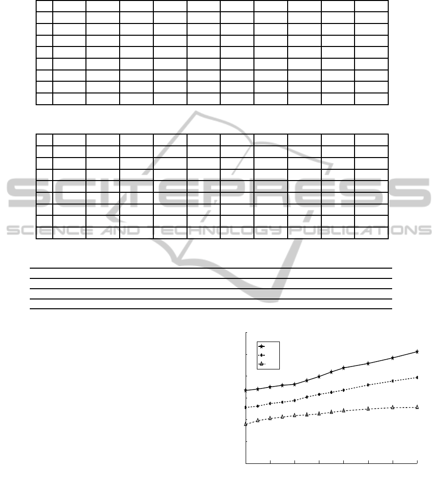
Table 5: Residual Energy(nJ) in each node of 8x10 Single Mobile Sink WSNs after 1386 iterations.
1 2 3 4 5 6 7 8 9 10
0 0.096 0.003 0.009 0.036 0.826 1.104 0.778 0.209 0.009 0.518
1 0.085 0.086 0.000 0.002 1.004 0.000 0.096 0.020 0.230 0.623
2 0.876 1.021 1.002 0.000 0.000 1.467 0.024 1.000 0.623 1.035
3 0.002 0.25 0.535 0.952 0.000 0.000 0.003 0.800 0.873 0.803
4 1.378 0.096 0.085 1.072 0.204 0.000 0.000 0.000 0.430 0.180
5 1.002 1.325 1.535 0.052 0.800 1.00 0.023 0.867 1.873 0.643
6 1.085 0.096 0.08 0.92 1.04 1.001 1.009 0.000 1.430 0.518
7 0.376 1.823 0.009 0.03 0.726 0.004 0.078 0.009 1.009 0.543
Table 6: Residual Energy(nJ) in each node of 8x10 Multiple Mobile Sink WSNs after 1646 iterations.
1 2 3 4 5 6 7 8 9 10
0 1.002 0.325 0.535 0.052 0.800 1.000 0.023 0.000 0.873 0.643
1 0.902 0.963 1.001 1.258 0.020 0.000 1.109 0.003 0.424 0.970
2 0.376 0.823 0.000 0.030 0.726 0.004 0.078 0.009 0.009 0.543
3 0.902 0.090 0.001 0.258 0.020 0.000 0.109 0.008 0.424 0.000
4 0.876 0.021 0.002 0.000 0.000 0.467 0.024 0.000 0.623 0.035
5 0.096 0.000 0.009 0.036 0.826 0.104 0.778 0.209 0.009 0.518
6 0.085 0.086 0.000 0.002 0.004 0.000 0.096 0.009 0.230 0.623
7 0.876 0.021 0.002 0.000 0.090 1.467 0.024 0.000 0.623 0.035
Table 7: Lifetime of the networks with Variable number of sensor nodes in a given area 100m x 100m.
Nodes 10 15 20 25 30 35 40 45 50 55 60 65 70 75 80
SS 143 298 452 547 667 713 760 778 804 824 856 889 904 910 914
SMS 276 438 618 734 868 964 1048 1099 1167 1201 1248 1298 1333 1346 1386
MMSS 354 556 739 866 996 1090 1179 1239 1296 1352 1398 1469 1528 1589 1646
formly and thus improves the lifetime of the network.
The selection of optimal number of mobile sinks
depend on the size and density of the network. When
the number of mobile sink increases to three, the net-
work lifetime is approximately equals to lifetime of
the network with two mobile sinks as shown in Figure
4. We can conclude that two mobile sinks are optimal
for the network with 80 nodes.
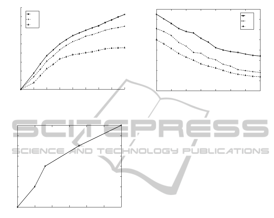
Figure 5 and 6 presence the lifetime of the MMSS,
SMS and SS. It is observed that the lifetime of MMSS
approach is higher than SMS and SS approaches.
While the lifetime of SS and SMS approach is 914
and 1386 time units, the lifetime of MMSS approach
is 1646 units i.e., 56% more than SS and 28% more
than SMS.
Figure 7 depicts the number of sinks required for
a variable number of sensors. It is observed that two
sinks are sufficient for nearly 100 sensor nodes and
there after there is a linear increase in the requirement
of sinks to maintain the desired performance of life-
time and delay.
Figure 8 shows plot of the graph for the delay and
number of sensor nodes with static sink, single mo-
bile sink and multiple mobile sinks. The simulation
10 20 30 40 50 60 70 80
10
15
20
25
30
35
40
Number of Sensor Nodes
Network lifetime (weeks)
MMSS
SMS
SS
Figure 5: Comparison of lifetime between the MMSS, SMS
and SS Networks.
starts with 10 sensor nodes to 80 nodes. Response
Time (delay) is calculated as per Equation 8. We ob-
serve that there is a considerable reduction in delay
for multiple mobile sink. This reduction of delay is
due to less number of hops and reduced distance be-
tween the source and the sink. In SS approach, the
average delay is 37 msec for 10 nodes while 30 msec
MULTIPLE MOBILE SYNCHRONISED SINKS (MMSS) FOR ENERGY EFFICIENCY AND
LIFETIMEMAXIMIZATION INWIRELESS SENSOR NETWORKS
83
0 10 20 30 40 50 60 70 80
0
200
400
600
800
1000
1200
1400
1600
1800
Number of Sensor Nodes
Number of Iterations
MMSS
SMS
SS
Figure 6: Comparison of number of iterations between the
MMSS, SMS and SS Networks.
0 50 100 150 200 250 300
0
0.5
1
1.5
2
2.5
3
3.5
4
Number of Sensor Nodes
Number of sinks
Figure 7: Number of nodes vs Number of sinks.
and 25msec respectively for SMS and MMSS ap-
proaches. Thus there is reduction in delay by 50% in
MMSS in comparison to SS. As the network density
increase, there is gradual reduction in average delay.
Though, there is large reduction in delay between SS
and SMS, but the reduction is much lower between
SMS and MMSS.
8 CONCLUSIONS
In WSN with a static sink, all source node forwards
data towards the sink. In a single mobile sink net-
work, sink moves to pre-determined positions and
stays for the sojourn time to collect the data. We
propose a distributed algorithm with Multiple Mobile
Synchronized Sink to improve the lifetime of the sen-
sor network. A linear program model is proposed to
increase the lifetime of the network and to reduce the
delay in the transmission of data between the source
10 20 30 40 50 60 70 80
0
5
10
15
20
25
30
35
40
Number of Sensor Nodes
Average Delay(msec)
SS
SMS
MMSS
Figure 8: Number of nodes vs Response Time (Delay).
node and the mobile sink nodes. For the proposed
model, simulation is carried out for multiple mobile
sink which increases the lifetime by 56% over single
static sink and 28% over single mobile sink network.
During the last iteration of MMSS WSN, the residual
energy of all the sensor nodes is almost same which
shows that energy drains uniformly and thus increases
the lifetime of the network. The proposed MMSS al-
gorithm minimizes the delay in the network at a very
small increase in cost of multiple mobile sinks. In
future, this can be developed for large scale WSNs
including reliability and recovery.
REFERENCES
Chang, J. and Tassiulas, L. (2000). Energy conserving rout-
ing in wireless ad-hoc networks. In IEEE INFOCOM,
pages 22–31.
Gandham, S., Dawande, M., Prakash, R., and Venkatesan,
S. (2003). Energy efficient schemes for wireless sen-
sor networks with multiple mobile base stations. In
IEEE GLOBECOM, volume 1, pages 377–381.
Gatzianas, M. and Georgiadis, L. (2008). A distributed al-
gorithm for maximum lifetime routing in sensor net-
works with mobile sink. In IEEE Transactions on
Wireless Communications, volume 7, pages 984–994.
Getsy, S. S., Kalaiarasi, R., Neelavathy, P. S., and Sridha-
ran, D. (November, 2010). Energy efficient clustering
and routing in mobile wireless sensor network. In In-
ternational Journal of Wireless & Mobile Networks,
volume 2.
Kusy, B., Lee, H., Wicke, M., Milosavijevic, N., and
Guibas, L. (April 13-16, 2009). Predictive qos rout-
ing to mobile sinks in wireless sensor networks. In
Proceedings of ISPN.
Luo, J. (2006). Mobility in wireless networks: Friend or
ICEIS 2011 - 13th International Conference on Enterprise Information Systems
84

foe, network design and control in the age of mobile
computing. In Ph.D. dissertation, EPFL,.
Luo, J., Panchard, J., Piorkowski, M., Grossglauser, M., and
Hubaux, J. P. (2005). Mobiroute: Routing towards a
mobile sink for improving lifetime in sensor networks.
In the National Conference Center in Research on Mo-
bile Information and Communication Systems(NCCR-
MICS).
Madan, R., Cui, S., Lall, S., and Goldsmith, A. (2005).
Cross-layer design for lifetime maximization in
interference-limited wireless sensor networks. In
IEEE INFOCOM, volume 3, pages 1964–1975.
Madan, R. and Lall, S. (2006). Distributed algorithms
for maximum lifetime routing in wireless sensor net-
works. In IEEE Transactions on Wireless Communi-
cations, volume 5, pages 2185–2193.
Michail, A. and Ephremides, A. (2003). Energy-efficient
routing for connection oriented traffic in wireless ad-
hoc networks. In Mobile Networks and Applications,
pages 517–533.
Weiwang, V. S. and Chua, K. C. (August 2005). Using mo-
bile relays to prolong the lifetime of wireless sensor
networks. In Proceeding of MOBICOM’05. Cologne,
Germany.
Xiao, L., Johansson, M., and Boyd, S. (2004). Simultane-
ous routing and resource allocation via dual decompo-
sition. In IEEE Transactions Community, volume 52,
pages 1136–1144.
Zhi, H., San-Yang, L., and Xiao-Gang, Q. (July 2010).
Overview of routing in dynamic wireless sensor net-
works. In International Journal of Digital Content
Technology and its Applications, volume 4.
MULTIPLE MOBILE SYNCHRONISED SINKS (MMSS) FOR ENERGY EFFICIENCY AND
LIFETIMEMAXIMIZATION INWIRELESS SENSOR NETWORKS
85
