TOWARD A NON INVASIVE CONTROL OF APPLICATIONS

A Biomedical Approach to Failure Prediction

Ilenia Fronza, Alberto Sillitti, Giancarlo Succi and Jelena Vlasenko

Free University of Bolzano, Bozen, Piazza Domenicani, Domenikanerplatz, 3, I-39100 Bolzano – Bozen, Italy

Keywords: Failure prediction, Survival analysis, Cox PH model, Event sequence data, Log files.

Abstract: Developing software without failures is indeed important. Still, it is also important to detect as soon as

possible when a running application is likely to fail, so that corrective actions can be taken. Following the

guidelines of Agile Methods, the goal of our research is to develop a statistical prediction model for failures

that does not require any additional effort on the side of the developers of an application; the key concept is

that the developers concentrate on the code and we use the information that is naturally generated by the

running application to assess whether an application is likely to fail. So the developers concentrate only on

providing direct value to the customer and then the model takes care of informing the environment of the

possible crash. The proposed model uses as input data that is commonly produced by developers: the log

files. The statistical prediction model employed comes from biomedical studies about cancer survival

prediction based on gene expression profiles where gene expression measurements and survival times of

previous patients are used to predict future patients' survival. One of the most prominent models is the Cox

Proportional Hazards (PH) model. In this work, we draw a parallel between our context and the biomedical

one; we consider types of operations as genes, and operations and their multiplicity in the sequence as

expression profiles. Then, we identify signature operations applying the above mentioned Cox PH model.

We perform a prototypical analysis using real-world data to assess the suitability of our approach. We

estimate the confidence interval of our results using Bootstrap.

1 INTRODUCTION

Moving from proactive maintenance to preventive

maintenance may reduce wastes caused by

downtime costs. Therefore, much of current research

is focused on predicting software failures with a

sufficient lead of time before actual failure.

Failure prediction models are usually built upon

historic data to predict the occurrence of failures. In

general, some predictor variables are collected or

estimated at the beginning of a project and fed into a

model. This approach is reasonable for traditional

processes.

One of the key guidelines of Agile Methods is to

consider feedback, since "it is rare to find control

without feedback, because feedback gives much

better control and predictability than attempting to

control complicated processes with predefined

algorithms" (Poppendieck and Poppendieck, 2003).

Therefore, an Agile failure prediction model is

required to use feedback to refine itself during the

development process.

Moreover, to cope and even accomodate Agile

Methods, a failure prediction model needs not to

require any additional effort on the side of the

developers of an application. Developers need to

eliminate waste of time and to concentrate on the

code providing direct value to the customer.

Therefore, failure prediction models are required to

inform of the possible crash using information that is

naturally generated by the running application.

Being cognizant of the mentioned challenges, the

key objective of our study can be outlined as

follows: we propose a new, incremental failure

prediction tool which uses data from previous

iterations to refine itself at every iteration.

Our idea is to use as input for the model data that

is commonly produced by developers: the log files.

These files contain a series of events marked with

their occurrence times. Thus, we deal with

prediction of failure event(s) based on the analysis

of event sequence data.

To this purpose, some techniques already exist

and can be classified into design-based methods and

data-driven rule-based methods. In a design-based

Fronza I., Sillitti A., Succi G. and Vlasenko J..

TOWARD A NON INVASIVE CONTROL OF APPLICATIONS - A Biomedical Approach to Failure Prediction.

DOI: 10.5220/0003493000830091

In Proceedings of the 13th International Conference on Enterprise Information Systems (ICEIS-2011), pages 83-91

ISBN: 978-989-8425-54-6

 2011 SCITEPRESS (Science and Technology Publications, Lda.)

method, the expected event sequence is obtained

from the system design and is compared with the

observed event sequence. A system logic failure can

be identified by use of this comparison. Untimed and

timed automata models, and untimed and timed Petri

net models have been proposed in (Chen et al., 2009,

Sampath et al., 1994, Srinivasan and Jafari, 1993);

time template models (Holloway 1996, Pandalai and

Holloway, 2000) establish when events are expected

to occur basing on timing and sequencing

relationships of events, which are generated from

either timed automata models (system design) or

observations of manufacturing systems. The major

disadvantage of these methods is that in many cases,

events occur randomly and thus there is no system

logic design information available.

Data-driven rule based methods do not require

system logic design information. These methods are

made of two phases: 1) identification of the temporal

patterns, i.e., the sequences of events that frequently

occur, and then development of prediction rules

based on these patterns (Agrawal 1996, Mannila et

al., 1997), and 2) prediction of the occurrence of a

failure event basing on the time relationships among

events (Dunham, 2003; Klemettinen 1999; Li et al.,

2007).

Survival analysis models have been also

proposed to solve this issues. Code metrics are given

as input to Cox PH model in (Wedel et al., 2008) to

analyze failure time data from bug reports of open

source software. In (Li et al., 2007) the Cox PH

model is used to predict system failures based on the

time-to-failure data extracted from the event

sequences. Only event combinations identified as

signatures are treated as explanatory variables in the

Cox PH model.

We propose a mechanism for lean, non invasive

control of applications. The idea is to build devices

that read logs of running applications and signal the

likely crash of such systems, thus adding no "muda"

(Liker 2003) to the development of each application.

We propose to collect (Dubson 2006) data using

Automated In-process Software Engineering

Measurement and Analysis (AISEMA) systems

(Coman et al., 2009). Then, we address the analyse

and decide phases (Dubson 2006) looking at

biological studies about cancer survival prediction

based on gene expression profiles. The idea is to

follow biomedical guidelines to:

 analyse data and identify signature operations of

failure;

 assign a risk score to future sequences of

operations;

 decide if these sequences will fail or not.

This mechanism looks at the running system as a

“black box”, meaning that we do not have any other

information about the system except the log files.

Altogether, the proposed approach is:

 lean, because there is no need of an explicit

mechanism on the applications (Liker, 2003);

 non-invasive, because data is collected by an

AISEMA system (Coman et al., 2009);

 intended to become an incremental failure

prediction tool which is built after each end of a

sequence of operations and uses data from previous

iterations to refine itself at every iteration.

In this work, we first draw a parallel between our

context and the biomedical one, since they deal with

different types of entities. As a result of this parallel,

we consider types of operations as genes, and

operations and their multiplicity in the sequence as

expression profiles. Signature operations of failures

are identified applying the Cox PH model, one of the

most prominent models in biomedical studies.

Then, we present a prototypical analysis using

real-world data, consisting in log files collected

during approximately 3 months of work in an

important Italian company that prefers to remain

anonymous. We propose to use Bootstrap methods

to determine the confidence interval of our results

The paper is structured as follows: in Section 2,

we present some background about survival analysis

together with the Cox Proportional Hazard (PH)

model and its applications; in Section 3, we

introduce our approach to failure prediction. In

Section 4, sample applications are presented. In

Section 5 we discuss our results.

2 BACKGROUND

2.1 Survival Analysis

The term “survival data” is used in a broad sense for

data involving time to the occurrence of a certain

event. The event of interest is usually death, the

appearance of a tumor, the development of some

disease, or some negative experience; thus, the event

is called “failure”. However, survival time may be a

positive event, like time to return to work after an

elective surgical procedure (Kleinbaum and Klein,

2005), or cessation of smoking, and so forth.

In the past decades, applications of the statistical

methods for survival data analysis have been

extended beyond biomedical research to other fields,

for example criminology (Benda, 2005; Schmidt and

Witte, 1989), sociology (Agerbo, 2007; Sherkat and

ICEIS 2011 - 13th International Conference on Enterprise Information Systems

Ellison, 2007), and marketing (Barros and Machado,

2010; Chen et al., 2009).

The study of survival data has previously

focused on predicting the probability of response,

survival, or mean lifetime, and comparing the

survival distributions of experimental animals or of

human patients.

In recent years, the identification of risk and/or

prognostic factors related to response, survival, and

the development of a disease has become equally

important (Persson, 2002).

The analysis of survival data is complicated by

issues of censoring. Censored data arises when an

individual’s life length only is known to occur in a

certain period of time (Kleinbaum and Klein, 2005).

2.2 The Cox Proportional Hazards

(PH) Model

Introduced by D.R. Cox in 1972 (Cox, 1972), the

semiparametric Cox PH model estimates the hazard

function, which assesses the instantaneous risk of

failure.

The data, based on a sample of size n, consists of

, t

, δ

), i = 1, ... , n where:

 x

is the vector of p covariates or risk factors for

individual i which may affect the survival

distribution of the time to event;

 t

is the time under observation for individual i;

 δ

is the event indicator (δ

=1 if the event has

occurred, δ

=0 otherwise).

The Cox PH model has became the most commonly

used model to give an expression for the hazard at

time t with a given specification of p covariates x:

(1)

The Cox PH model formula says that the hazard at

time t is the product of two quantities:

 the baseline hazard function h

(t), which is equal

for all the individuals. It may be considered as a

starting version of the hazard function, prior to

considering any of the x´s;

 the exponential expression e to the linear sum of

, where the sum is over the p explanatory x

variables.

The Cox PH model focuses on the estimation of the

vector of regression coefficients β leaving the

baseline hazard unspecified. In the p < n setting

(Bøvelstad, 2010), β´s are estimated by maximizing

the log partial likelihood, which is given by:

(2)

The key assumption of the Cox PH model is

proportional hazards; this assumption means that the

hazard ratio (defined as the hazard for one individual

over the hazard for a different individual) is constant

over time.

This model is widely used because of its

characteristics:

 even without specifying h

(t), it is possible to

find the β´s;

 no particular form of probability distribution is

assumed for the survival times. A parametric

survival model is one in which survival time (the

outcome) is assumed to follow a known distribution.

The Cox PH model is not a fully parametric model.

Rather it is a semi-parametric model because even if

the β's are known, the distribution of the outcome

remains unknown;

 it uses more information than the logistic model,

which considers a (0,1) outcome and ignores

survival times and censoring. Therefore it is

preferred over the logistic model when survival time

is available and there is censoring (Kleinbaum and

Klein, 2005).

2.3 Applications of the Cox PH Model

The Cox PH model was first used in biomedical

applications (Collett, 1994), mainly to determine

prognostic factors that affect the survival time of

patients to some type of diseases (mostly cancers)

(Eliassen et al., 2010, Pope et al., 2002).

After the completion of DNA sequencing, the

Cox PH model has been applied to gene expression

data to detect novel subtypes of a disease, or to

explore the potential associations between the high-

dimensional gene expression data and some clinical

outcome.

Cancer patient survival based on gene expression

profiles is an important application of genome-wide

expression data. The goal is to identify the optimal

combination of the gene expression data in

predicting the risk of cancer death.

The most common approach to model covariate

effects on cancer survival is the Cox PH model,

which takes into account the effect of censored

observations (Bøvelstad et al., 2007, Hao et al.,

2009, Yanaihara et al., 2006, Yu et al., 2008). Gene

expression measurements and survival times of

previous patients are used to obtain a prediction rule

that predicts the survival of future patients.

TOWARD A NON INVASIVE CONTROL OF APPLICATIONS - A Biomedical Approach to Failure Prediction

Given n patients diagnosed with a specific type

of cancer, for each of the n patients the observations

, t

, δ

) are available, where:

 x

= (x

, … , x

) contains the measurements of p

gene expression values for patient i; i = 1, ... , n;

 t

is the time under observation of patient i;

 the censoring index δ

keeps track of whether

patient i died (δ

= 1) or was censored (δ

= 0), i.e.,

patient i was still alive at the end of the study or if

she or he dropped out of the study or died from

another cause.

Applications of the Cox PH model can be found in

several fields of research other than biomedicine,

such as criminology (Benda, 2005; Schmidt and

Witte, 1989), sociology (Agerbo, 2007; Sherkat and

Ellison, 2007), marketing (Barros and Machado,

2010; Chen et al., 2009), and cybernetic (Li et al.,

2007). There is also an application of the Cox PH

model to software data in (Wendel 2008) where,

using as input code metrics, failure time data coming

from bug reports have been analysed.

2.4 The Bootstrap Method

In statistics the average is often used to guess the

overall behavior of a population using the

information coming from a sample; depending on

the structure of the population, the average could

then be implemented by taking the means, the

median, or the mode (Fisher and Hall, 1991).

However, it is interesting also to know how reliable

is an estimate done with the average. To this end,

other statistical properties are often used, based on

the structure of the population (e.g., standard

deviations, percentiles, histograms). Clearly, a

reliable estimation of the confidence interval can

provide a very valuable information to the user of an

estimation.

To this end the Bootstrap technique has been

devised (Efron, 1987). Bootstrap is a computer-

based (it can be both parametric and non-parametric)

method to compute estimated standard errors,

confidence intervals, and hypothesis testing (Efron

and Tibshirani, 1993).

The Bootstrap algorithm first creates n datasets

of the same size of the original sample by randomly

picking elements of it with replacement; this

technique is called resampling. The number of the

generated sets needs to be high; a suitable number

could be 1000.

Then, the Bootstrap algorithm computes the

averages of each of the newly generated datasets –

the specific kind of average depends from the

statistical properties of the population. The results

are then used to determine the confidence interval of

the population from which the original sample was

drawn.

In this study we want to determine the reliability

of our estimations for failures. However, we have a

very limited dataset and we do not know the

parameters of the random variables of interest, and

the overall transformations are non-linear.

Therefore, we propose to use Bootstrap method.

Each time an estimation of failure or success is

done, we use Bootstrap to determine the reliability

of it, that is, the percentage of times in which the

results remain consistent with the original

prediction.

3 APPROACH

3.1 Schema of the Approach

To build devices that read logs of running

applications and signal the likely crash of such

systems, we have to address the four main activities

reported in (Dobson et al., 2006): 1) collect, 2)

analyse, 3) decide, and 4) act.

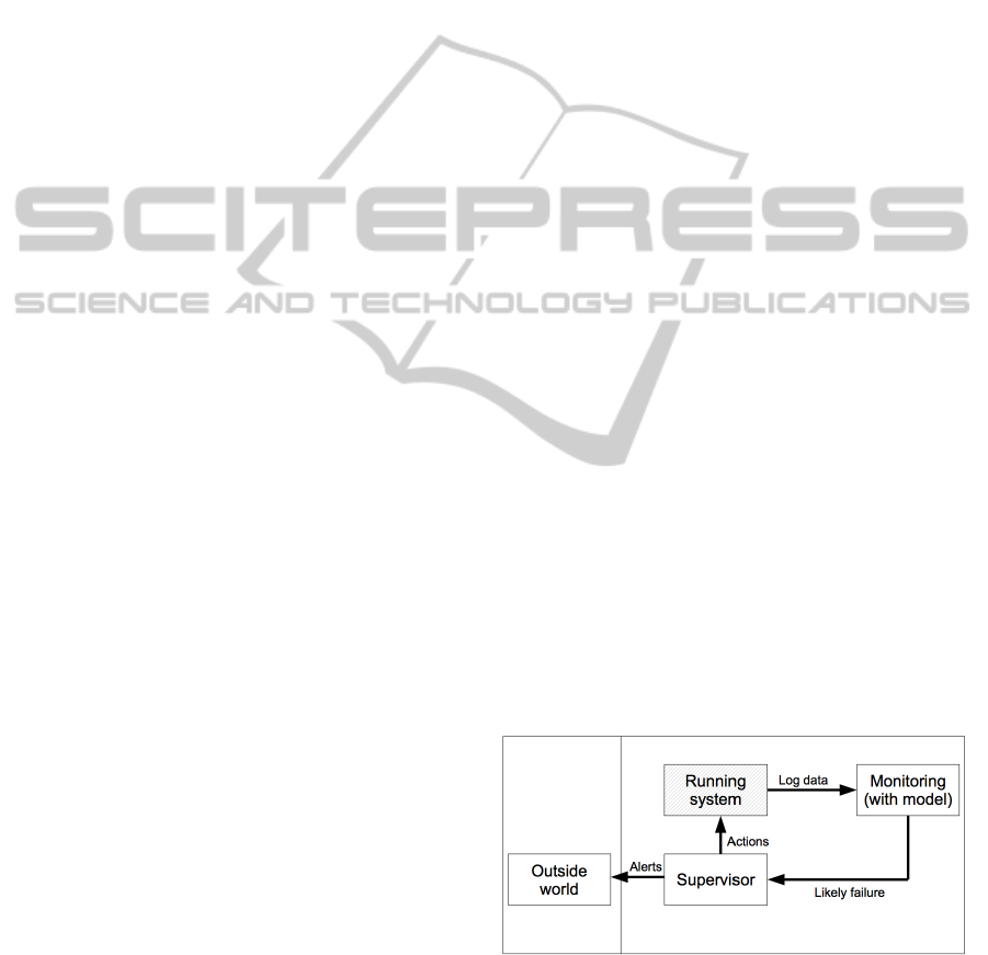
Figure 1 presents a schematic view of the

proposed approach.

While the system is running, an AISEMA system

(Coman et al., 2009) collects data to track the actual

execution path. In this work, we look at the running

system as a “black box”, meaning that we do not

have any other information about the system except

the log files.

The monitoring process takes log data as input,

analyses them, and basing on the analysis performed

decides the “likely failure” of the running

application and gives to the supervisor a message.

Figure 1: Schema of the devices that read logs of a

running system and signal the likely failure.

The supervisor can act directly on the running

system to avoid the predicted failure, or send an alert

to the outside world. Possible actions could be to

ICEIS 2011 - 13th International Conference on Enterprise Information Systems

abort the running system, to restart it, to dynamically

load components, or to inform the running system if

it was a suitably structured autonomic system

(Müller et al., 2009).

The monitoring process is based on the Cox PH

model. Our context seems to have the characteristics

needed to apply Cox PH model; in fact, survival

time and censored observations are available.

Moreover, the Cox PH model needs no assumption

of a parametric distribution for the event sequence

data. Therefore, we can benefit of the following

advantages:

 we can discover information that may be hidden

by the assumption of a specific distribution (Yu et

al., 2008);

 we obtain results comparable to the parametric

model even without this assumption (Kalbfleisch

and Prentice, 2002).

Our context is completely different from the

biomedical one. Therefore, before applying the Cox

PH model, we first drew a parallel between the two

contexts to provide an interpretation of the

biomedical entities in our case.

3.2 Parallel between Our Context and

the Biomedical One

The idea behind biomedical studies is that different

gene expression profiles may result in different

survival times. In software processes, the activities

performed may affect the time of survival to a

failure. Therefore, in our context, types of operations

in some sense play the role of genes.

The expression profile may be formed by each

operation's multiplicity, since it provides

information about the level of presence of the

operation.

Time under observation of a sequence is defined

as its length in terms of time, meaning that we

evaluate it as the difference between the time stamp

of the last operation and the time stamp of the first

operation in the sequence.

In our case, the “observed event” is the end of

the sequence because of a failure. Therefore, we

have the following definition: δ

=1 if i is a failure, δ

=0 otherwise.

Our type of censoring is type II with a

percentage of 100% (Lee and Wang, 2003), meaning

that δ

is never equal to zero because of the end of

the period of observation.

Table 1 summarizes the interpretation of

biological entities in our context. In biomedical

studies, gene expression measurements and survival

times of previous patients are used to obtain a

prediction rule that predicts the survival of future

patients. In this work, we consider types of

operations as genes, and operations and their

multiplicity in the sequence as expression profiles.

Table 1: Parallel between our context and the biomedical

one.

Variable Biological data Our data

Time under

observation of

patient i

Time under

observation of

sequence i (last

date – first date)

=1 if survival

time is observed

=0 elsewhere

=1 for failures

=0 elsewhere

, …, x

)

is the

expression value

of gene j in

patient i

is the

multiplicity of

operation j in

sequence i

i=1, …, n j=1, …, p

3.3 Structure of the Monitoring

Process

3.3.1 Dimensional Reduction of the Problem

Our method consists of the following steps to get

from raw logs to temporal event sequences (Zheng

et al., 2009) to be used as input for the analyses:

 data are parsed to extract operations together

with their associated time stamps and severities for

each event in the log file;

 duplicate rows are deleted together with logs that

are missing information in one or several of the

fields Operation, Time stamp, Severity;

 sequences of activities are extracted: a new

sequence starts either if there is a “Log in” operation

or if the day changes.

Failures are defined as sequences containing at least

one severity “Error”. Table 2 summarizes the

definitions used in this work.

Table 2: Definitions used in this work.

Notion Definition

sequence A chronologically ordered set of log entries

in the maximum time frame of 1 day. Two

sequences during the same day are

separated by a “Log in” operation

Failure A sequence containing at least one severity

“Error”

TOWARD A NON INVASIVE CONTROL OF APPLICATIONS - A Biomedical Approach to Failure Prediction

3.3.2 Preparation of the Input for the Cox

PH Model

Each temporal event sequence i is described by (x

, δ

), where:

 x

= (x

, ..., x

), and x

is the multiplicity of

operation j in sequence i;

 t

is the lifetime of the sequence, defined as the

difference between the last time stamp and the first

time stamp of sequence i;

 δ

= 1 when the event is “observed” (failure

sequences) and δi = 0 elsewhere (censored

observations).

3.3.3 Training of the Model

We propose to follow the guidelines given in

biomedical studies (Bøvelstad et al., 2007, Hao et

al., 2009, Yanaihara et al., 2006, Yu et al., 2008) to

analyse data about past sequences and decide about

the likely failure of the current sequence of

operations of the running system. In particular, the

training of the monitoring process includes the

following steps:

 the Schoenfeld test (Hosmer et al., 2008;

Kalbfleisch and Prentice, 2002; Kleinbaum and

Klein, 2005) is applied to select the operations

satisfying the PH assumption;

 hazard ratios from a multivariate Cox PH model

are used to identify which operations are associated

to a failing end of sequences. The k operation

included in the model are those operations whose

multiplicity in the sequence is expected to be related

to failure. Protective operations are defined as those

with hazard ratio for failure lower than 1. High-risk

operations are defined as those with hazard ratio for

failure greater than one;

 the k-operations signature risk score RS is

assigned to each sequence in the dataset, according

to the exponential value of a linear combination of

the multiplicity of the operation, weighted by the

regression coefficients derived from the

aforementioned Cox PH model;

 the following values are extracted: 1) m, the third

quartile of risk scores of non failure sequences, and

2) M, maximum risk score of non failure sequences.

3.3.4 Deciding the “Likely Failure” and the

Associated Confidence Interval

The k-operations signature risk score RS is evaluated

for the new sequence, and basing on its value the

sequence is defined as:

 “likely no failure” if RS ≤ m;

 “likely failure” if RS ≥ M;

 “still unknown” if m < RS < M.

In order to compute estimates of confidence

intervals of our dataset we propose to use the

Bootstrap method of resampling. We perform a

Bootstrap of 1000 times on the original data and

then we consider for each sequence the resulting

prediction.

The sets of the predictions is then used to

determine the likelihood of correctness of the

original prediction.

4 SAMPLE APPLICATIONS

To assess the suitability of our approach, we have

performed two prototypical analysis intended to

determine if it is worth pursuing the approach

further. We use two datasets consisting of log files

collected during approximately 3 months of work in

an important Italian company that prefers to remain

anonymous.

We prepared each dataset as discussed in Section

3.3.1 and Section 3.3.2. Then we assigned randomly

the sequences to training set (60%) or test set (40%).

Afterwards, we proceeded as discussed in Section

3.3.3 and Section 3.3.4 to 1) identify the k signature

operations of failure in the training set, 2) compute

the values of m and M, 3) assign the the k-operations

signature risk score to each sequence in the test set,

and 4) decide the “likely failure” of the sequences in

the test set.

4.1 First Sample

Table 3 contains the training set pre-processing

summary of the first sample

Table 3: Training set pre-processing summary (first

sample).

Notion Definition N %

Cases

available in

the analysis

Event

28 12.9

Censored 157 72.0

Total 185 84.9

Cases

dropped

Censored before the first

event in the stratum

33 15.1

Total 218 100

Dependent variable: survival time

Six out of the eight initial operations were

satisfying the proportional hazards assumption and

were therefore kept in the input dataset for the Cox

PH model. Three out of the six initial operations

ICEIS 2011 - 13th International Conference on Enterprise Information Systems

were kept in the output of the model. Table 4

contains the output of this model, together with the

definition of each operation as “protective” (or

“high-risk”) according to the exponential value of

the regression coefficient β.

Table 4: Output of Cox PH model on training set (first

sample).

β Sig Exp(β) definition

Operation 1 -0.40 0.013 0.961 Protective

Operation 2 0.06 0.015 1.006 High-risk

Operation 3 -0.52 0.055 0.592 protective

-2 Log Likelihood: 200.112

The comparison between failures and non

failures shows that higher risk scores have been

assigned to failure sequences (Figure 2).

Figure 2: Risk scores in failure and non-failure sequences

(first sample).

Altogether we obtained a value of m = 0.59 and

M = 1.85.

In the test set, the comparison of the risk scores

with m and M provides the following results: in 40%

of the cases the system is able to predict correctly

the failure and only in 1% of the cases a predicted

failure is not a failure, which means that a message

of expected failure is quite reliable. On the contrary,

the prediction of non-failure is not as reliable. 50%

of the failing sequences are predicted as non-failing.

4.2 Second Sample

Table 6 contains the training set pre-processing

summary of the second sample.

Table 5: Training set pre-processing summary (second

sample).

Notion Definition N %

Cases

available in

the analysis

Event

139 1.8

Censored 7445 98.2

Total 7584 100

Cases

dropped

Censored before the first

event in the stratum

0 0

Total 7584 100

Dependent variable: survival time

Six out of the ten initial operations were

satisfying the proportional hazards assumption and

were therefore given as input to the Cox PH model.

Two out of the six initial operations were kept in the

model. Table 7 contains the output of this model,

together with the definition of each operations as

“protective” (or “high-risk”) according to the

exponential value of the regression coefficient β.

Table 6: Output of the Cox PH model on the training set

(second sample).

β Sig Exp(β) definition

Operation 1 0.66 0.001 1.925 High-risk

Operation 2 0.32 0.001 1.380 High-risk

-2 Log Likelihood: 1746.471

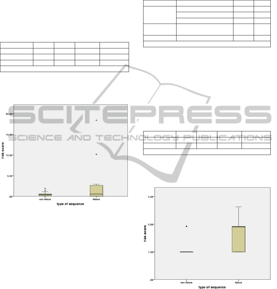
The comparison between failures and non

failures shows that higher risk scores have been

assigned to failure sequences (Figure 3).

Figure 3: Risk scores in failure and non failure sequences

(second sample).

In this case, we obtain a value of m = 1.00 and M

= 1.93.

In the test set, the comparison of the risk scores

with m and M provides the following results: in

100% of the cases the approach taken is able to

predict correctly the failure, and in 99.6% of the

cases the system is able to predict correctly the non

TOWARD A NON INVASIVE CONTROL OF APPLICATIONS - A Biomedical Approach to Failure Prediction

failure. Both the messages of expected failure and

non failure appear to be quite reliable.

5 CONCLUSIONS

In this work we propose a mechanism for lean, non

invasive control of applications. We use an

AISEMA system (Coman et al., 2009) to collect

data; then we apply the Cox PH Model following the

biomedical guidelines to find the k signature

operations of failure and to decide about the “likely

failure” of future sequences

Altogether, the proposed approach presents the

following advantages:

 it is lean, because there is no need for an explicit

mechanism on the application;

 it is non invasive, because data is collected using

AISEMA systems;

 data collection is low cost;

 measurement is continuous and accurate;

 developers' efficiency is not affected by data

collection since they can concentrate on their tasks

as usual.

The proposed mechanism is intended to become an

incremental failure prediction tool which is built

after each end of a sequence of operations and

refines itself at every iteration using data from

previous iterations.

Results from our preliminary, prototypical

analysis appear quite interesting and worth further

investigations; higher risk scores are assigned to

failure sequences in the test set. Overall, the

proposed approach appears very effective in the

identification of True Positives and True Negatives,

meaning that the sequences identified as leading to a

failure are very likely to lead to a failure.

Additional work is now needed to use Bootstrap

methods to determine the confidence interval of our

results; we are now accomplishing this task.

Moreover, we need to study more in-depth our

promising mechanism to determine the

generalizability of our results. To this end, we are

going to study more in-depth our model, trying to

generalize our results. In particular, we plan to

replicate the analysis on more industrial datasets.

We are also considering the following

approaches to achieve higher levels of precisions: 1)

the Cox PH model with strata to analyse covariates

not satisfying the PH assumption, 2) specific

techniques to manage datasets with a limited number

of cases (Bøvelstad, 2010), and 3) application of

Bootstrap methods in order to identify the

confidence interval of the prediction.

We should also investigate how other “black-

box” properties of applications (e.g., memory usage,

number of open files, processor usage) can be

considered to predict failures.

We will also deal with the bias introduced when

calculating survival time without considering the

duration of the last operation.

We will then try to predict a failure analysing

only an initial portion of a sequence, to obtain an

early estimation of failure, providing additional time

to take corrective actions.

Finally, the proposed model could be particularly

useful dealing with autonomic systems (Müller et

al., 2009).

ACKNOWLEDGEMENTS

We thank the Autonomous Province of South Tyrol

for supporting us in this research.

REFERENCES

Agerbo, E. 2007. High Income, Employment,

Postgraduate Education, and Marriage: a Suicidal

Cocktail among Psychiatric Patients. Archives of

General Psychiatry, 64, 12, 1377-1384.

Barros, C. P. and Machado, L. P. 2010. The Length of

Stay in Tourism. Annals of Tourism Research, 37, 3,

692-706.

Benda, B. 2005. Gender Differences in Life-Course

Theory of Recidivism: A Survival Analysis.

International Journal of Offender Therapy and

Comparative Criminology, 49, 3, 325-342.

Bøvelstad, H. M., Nygård, S., Størvold, H. L., Aldrin, M.,

Borgan, Ø., Frigessi, A., and Lingjærde, O. C. 2007.

Predicting Survival from Microarray Data: a

Comparative Study. Bioinformatics, 23, 16, 2080-

2087.

Bøvelstad, H. M. 2010. Survival Prediction from High-

Dimensional Genomic Data. Doctoral Thesis.

University of Oslo.

Chen,Y., Zhang, H., and Zhu, P. 2009. Study of Customer

Lifetime Value Model Based on Survival-Analysis

Methods. In World Congress on Computer Science

and Information Engineering (Los Angeles, USA,

March 31 – April 02, 2009), 266-270.

Coman, I. D., Sillitti, A., and Succi, G. 2009. A case-study

on using an Automated In-process Software

Engineering Measurement and Analysis system in an

industrial environment. In ICSE’09: International

Conference on Software Engineering (Vancouver,

Canada, May 16-24 May, 2009), pp. 89-99.

ICEIS 2011 - 13th International Conference on Enterprise Information Systems

Cox, D.R. 1972. Regression models and life-tables.

Journal of the Royal Statistical Society Series B, 34,

187-220.

Collett, D. 1994. Model ling Survival Data in Medical

Research. Chapman&Hall, London.

Dobson, S., Denazis, S., Fernández, A., Gaiti, D.,

Gelenbe, E., Massacci, F., Nixon, P., Saffre, F.,

Schmidt, N., and Zambonelli, F. 2006. A Survey of

Autonomic Communications. ACM Transactions on

Autonomous and Adaptive Systems, 1, 2, 223-259.

Efron, B. 1987. Better Bootstrap Confidence Interval.

Journal of the American Statistical Association, 82,

171-200.

Efron, B. and Tibshirani, R.: An Introduction to the

Bootstrap. Chapman & Hall (1993).

Eliassen, A. H., Hankinson, S. E, Rosner, B., Holmes, M.

D., and Willett, W. C. 2010. Physical Activity and

Risk of Breast Cancer Among Postmenopausal

Women. Archives of Internal Medicine, 170, 19, 1758-

1764.

Fisher, N. I. and Hall, P. 1991. Bootstrap algorithms for

small samples. Journal of Statistical Planning and

Inference, 27, 157-169.

Hao, K., Luk, J. M., Lee, N. P. Y., Mao, M., Zhang, C.,

Ferguson, M. D., Lamb, J., Dai, H., Ng, I. O., Sham,

P.C., and Poon, R.T.P. 2009. Predicting prognosis in

hepatocellular carcinoma after curative surgery with

common clinicopathologic parameters. BMC Cancer,

9, 398-400.

Hosmer, D. W., Lemeshow, S., and May, S. 2008. Applied

survival analysis: Regression modeling of time to

event data. Wiley.

Kalbfleisch, J. D. and Prentice, R. L. 2002. The statistical

analysis of failure time data. Wiley.

Kleinbaum, D. G. and Klein, M. 2005. Survival analysis:

a self-learning test (Statistics for Biology and Health).

Springer.

Lee E. T. and Wang, J. W. 2003. Statistical methods for

survival data analysis. Wiley.

Li, Z., Zhou, S., Choubey, S., and Sievenpiper, C. 2007.

Failure event prediction using the Cox proportional

hazard model driven by frequent failure sequences.

IEE Transactions, 39, 3, 303-315.

Liker, J. 2003. The Toyota Way. 14 Management

Principles from the World's Greatest Manufacturer.

McGraw Hill.

Mannila, H., Toinoven, H., and Verkamo, A. I. 1997.

Discovery of frequent episodes in event sequences.

Data Mining and Knowledge Discovery, 1, 259-289.

Müller, H. A., Kienle, H. M., and Stege, U. 2009.

Autonomic Computing: Now You See It, Now You

Don’t—Design and Evolution of Autonomic Software

Systems. In: De Lucia, A., Ferrucci, F. (eds.):

Software Engineering International Summer School

Lectures: University of Salerno 2009. LNCS, vol.

5413, pp. 32-54. Springer-Verlag.

Pandalai, D. N. and Holloway, L. E. 2000. Template

languages for fault monitoring of timed discrete event

processes. IEEE Transactions on Automatic Control

45, 5, 868-882.

Persson, I. 2002. Essays on the Assumptions of

Proportional Hazards in Cox Regression. Doctoral

Thesis. Uppsala University.

Pope, C. A., Burnett, R. T., Thun, M. J., Calle, E. E.,

Krewski, D., Ito, K., and Thurston, G. D. 2002. Lung

Cancer, Cardiopulmonary Mortality, and Long-term

Exposure to Fine Particulate Air Pollution. Journal of

the American Medical Association, 27, 9, 1132- 1141.

Poppendieck, M. and Poppendieck, T. 2003. Lean

software development: an Agile toolkit. Addison

Wesley.

Sampath, M., Sengupta, R., and Lafortune, S. 1994.

Diagnosability of discrete event systems. In:

International Conference on Analysis and

Optimization of Systems Discrete Event Systems

(Sophia, Antipolis, June 15 – 17, 1994), pp. 73-79.

Schmidt, P. and Witte, A. D. 1989. Predicting Criminal

Recidivism Using “Split Population” Survival Time

Models. Journal of Econometrics, 40, 1, 141-159.

Sherkat, D. E. and Ellison, C. G.: Structuring the Religion-

Environment Connection: Religious Influences on

Environmental Concern and Activism. Journal for the

Scientific Study of Religion, 46, 71-85 (2007).

Srinivasan, V. S. and Jafari, M. A. 1993. Fault

detection/monitoring using time petri nets. IEEE

Transactions on System, Man and Cybernetics, 23, 4,

1155-1162.

Wedel, M., Jensen, U., and Göhner, P. 2008. Mining

software code repositories and bug databases using

survival analysis models. In: 2nd ACM-IEEE

international symposium on Empirical software

engineering and measurement (Kaiserslautern,

Germany, October 09 - 10, 2008), pp. 282-284.

Yanaihara, N. et al. 2006. Unique microRNA molecular

profiles in lung cancer diagnosis and prognosis.

Cancer Cell, 9, 3, 189-198.

Yu, S. L. et al. 2008. MicroRNA Signature Predicts

Survival and Relapse in Lung Cancer. Cancer Cell,

13, 1, 48-57.

Zheng, Z., Lan, Z., Park, B. H., and Geist, A. 2009.

System log pre-processing to improve failure

prediction. In: 39th Annual IEEE/IFIP International

Conference on Dependable Systems & Networks

(Lisbon, Portugal, June 29 – July 2), pp. 572-577.

TOWARD A NON INVASIVE CONTROL OF APPLICATIONS - A Biomedical Approach to Failure Prediction