
BANGLA ISOLATED WORD SPEECH RECOGNITION
Adnan Firoze, M. Shamsul Arifin, Ryana Quadir and Rashedur M. Rahman
Department of Electrical Engineering and Computer Science, North South Univeristy, Bashundhara, Dhaka, Bangladesh
Keywords: Speech Recognition, Spectrogram, Fuzzy Logic, STFT, Standard Deviation, Segmentation.
Abstract: The paper presents Bangla word speech recognition using spectral analysis and fuzzy logic. As human
speech is imprecise and ambiguous, the fuzzy logic – the base of which is indeed linguistic ambiguity, could
serve as a more precise tool for analysing and recognizing human speech. Even though the core source of an
uttered word is a voiced signal, our system revolves around the visual representation of voiced signals – the
spectrogram. The spectrogram may be perceived as a “visual” entity. The essences of a spectrogram are
matrices that include information about properties of a sound, e.g., energy, frequency and time. In this
research the spectral analysis has been chosen as opposed to image processing for increased accuracy. The
decision making process of our system is based on fuzzy logic. Experimental results demonstrate that our
system is 80% accurate compared to a commercial Hidden Markov Model (HMM) based speech recognizer
that shows 73% accuracy on an average.
1 INTRODUCTION
Human speech recognition has a broader solution
which refers to the technology that can recognize
speech. The recognition process is still open because
none of the current methods are fast and precise
enough compared to human recognition abilities.
Research in this area has attracted a great deal of
attention over the past five decades. Several
technologies are applied and efforts were made to
increase the performance up to marketplace standard
so that the users will have the benefit in a variety of
ways.
During this long research period several key
technologies were applied to recognize isolated
words such as Hidden Markov Models (Abul et al.,
2007), Artificial Neural Networks (ANN), Support
Vector Classifiers with HMM, Independent
Component Analysis, HMM and Neural-Network
Hybrid, the stochastic language model and more
(Juang and Rabiner, 2005).
On recognizing Bangla speech, most of the
research efforts had been performed using the ANN
based classifier. But no research work has been
reported that uses the Fuzzy logic, MEL filtering and
STFT methods. Therefore, in this research we
investigated, proposed and implemented a model
that could recognize Bangla isolated words by using
fuzzy logic and spectral analysis.
The ambiguity in phonemes in Bengali speech is
more intense and varied than that of English speech
since Bangla stems from the “Indo-European
language family” just as Hindi, Urdu, Persian and
numerous languages from South Asia having native
speakers of over 3 billion (Weiss, 2006). Therefore
our approach for speech recognition considers the
“word level” rather than the “phonetic level.” In
other words the base or smallest entity of our system
is a “word” (in Bangla) rather than a sound
(phoneme) that constructs the words. We also want
to mention that HMM based speech recognizers
work from the phonetic level as opposed to “word
level” since most of the HMM based systems are
optimized for English speech.
In our Fuzzy Inference System (FIS), we have
taken three inputs, i.e., frequency, energy level of
the sample, and the energy level of the target or
description. Since human ear is more susceptible to
lower frequencies of sounds, our FIS rules are made
accordingly to put emphasize on the lower
frequencies. The output of our FIS is the similarity
between two “segments” of a word and the overall
evaluation of the FIS has been cumulated to reach
the verdict of word recognition.
The organization of the paper is as follows:
Section 2 discusses the related works done till date
in relevance to speech recognition emphasizing on
Bangla speech (phoneme descriptions, vowels and
recognition systems) in particular. Section 3 presents
73
Firoze A., Arifin M., Quadir R. and Rahman R..
BANGLA ISOLATED WORD SPEECH RECOGNITION.
DOI: 10.5220/0003492700730082
In Proceedings of the 13th International Conference on Enterprise Information Systems (ICEIS-2011), pages 73-82
ISBN: 978-989-8425-54-6
Copyright
c
2011 SCITEPRESS (Science and Technology Publications, Lda.)

the detailed descriptions about the strategies that we
implement to build our system. In Section 4 we
report and analyze the experimental results. Finally,
Section 5 concludes giving future directions of our
research.
2 RELATED WORKS
Even though Speech Recognition is still an open
problem with quite low accuracy, the attempt to
recognize speech dates back to the 1950s. The very
first speech recognizer only recognized digits that
were spoken (Davies et al., 1952). After the first
attempt the speech recognition was centered on
voice commands in devices and utility services. In
1990 AT&T call centre service devised the first
command recognition. When customers called their
help lines they could give voice instructions (Juang
and Rabiner, 2005). However this attempt was not
successful since most dialects could not be
recognized.
Since then approaches were revolved around the
visual representation of speech. Documentation of
the relationship between a given speech spectrum
and its acoustic properties were done in 1922 by
Fletcher and others at the Bell Laboratories
(Fletcher, 1922). Thus Harvey Fletcher became one
of the pioneers in recognizing the importance of the
spectral analysis in detecting phonetic attributes of
sound.
Even though the attempts to recognize human
speech properly goes a long period back in time, the
speech recognition approaches in Bangla language
started only in the 21
st
century. In a research work
(Roy et al., 2002), performed the recognition by
ANN using Back propagation Neural Network. A
phoneme recognition approach using ANN as a
classifier was devised in (Hassan el al., 2003). RMS
energy level was calculated by them as feature from
the filtered digitized signal. In (Karim et al., 2002)
authors presented a technique to recognize Bangla
phonemes using Euclidian distance measure.
Authors in (Rahman et al., 2003) presented
continuous Bangla speech segmentation system
using ANN where reflection coefficient and
autocorrelations were used as features. They applied
Fourier transform based spectral analysis to generate
the feature vectors from each isolated words.
Authors (Islam et al, 2005) presented a Bangla ASR
system that employed a three layer back propagation
Neural Network as the classifier. In a research paper
Hasnat and others (Abul et al., 2007) presented an
HMM based approach in recognizing both isolated
and continuous Bangla speech recognition using
HMM models and MFCC.
3 METHODOLOGY
The main goal in this research is to create a platform
that could translate Bengali speech to Bengali text
through proper recognition by spectrogram and
fuzzy logic. However to do so, first we need to train
the computer-system in a fuzzy learning
methodology with original or correct form of
utterance of words. Our strategy is divided into two
major phases: Learning phase and Recognition
phase. Each of the phases consists of multiple steps.
Even though the phases are named differently, some
of the steps overlap with each other. They are
vividly illustrated by the flowchart presented in
Figure 1.
3.1 Recording Speech
The first step is self explanatory. We first get input
speech in our system. Our system could work on
previously recorded “WAV” files or record speech
in real time. All sounds that we used and recorded
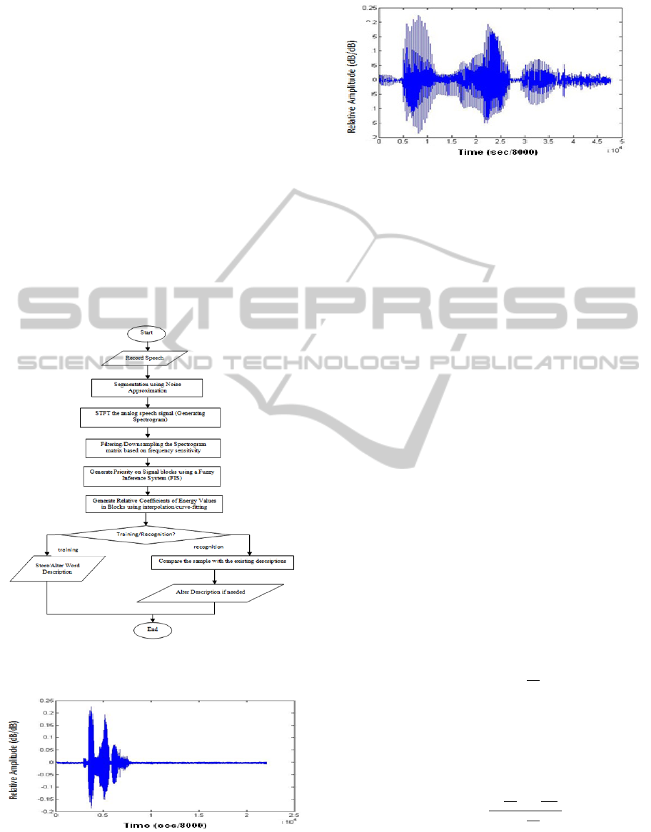
have the following specifications:
Bit-depth: 8 bit (7 KB/sec)
Bit-rate: 8.000 KHz
As the bit rate is 8 KHz we represent the “time
parameter” axes in “sec/8000” units in figures 2, 3.
Channel: mono (since we recognize speech,
the choice of dual-channel/stereo is meaningless as
both channels will give the same signal to our
system.)
3.2 Segmentation using Noise
Approximation
Before analysing further, it is imperative that data
speech and the descriptions stored in our database
need to be phased in such a way that one can be
superimposed onto the other. Simply put, if one
speaker starts to speak a word after two seconds
whereas the description in our database/dictionary
starts the data instantaneously then the two
descriptions will not superimpose properly.
Therefore, segmentation needs to be done in a way
such that both of the descriptions start from the same
point of time. This has been implemented with the
following way: when a speaker speaks a word, the
system will seek for the level where the amplitude of
the signal is greater than 0.2 dB/dB (relative
threshold amplitude that we approximate is based on
ICEIS 2011 - 13th International Conference on Enterprise Information Systems
74
noise of surroundings). A raw and segmented word
is presented in Figure 2 and Figure 3 respectively.
It should be mentioned that in the figures we use
the unit (dB/dB) to relate the “relative amplitude.”
The term “relative amplitude” that we use in this
research is the raw value of the energy level and the
relation of the “relative amplitude” with the
conventional decibel (dB) is expressed by the
following equation.
y=10log
10
(x) (1)
where, x = the relative amplitude
y = amplitude in decibel (dB)
Our system considers the signals that are greater
than the threshold value. It will end seeking when
the level goes below the threshold level of noise.
Thus we will find the interval between which the
speech exists and create description/compare with
database based on that segment of the word.
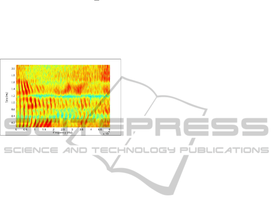
Figure 1: A Flowchart showing the methodology of the
system.
Figure 2: A raw (unsegmented) audio signal for the word
“Bangladesh”.
Figure 3: A segmented audio signal for the word
“Bangladesh”.
3.3 STFT (Short-time Fourier
Transform) the Speech
Data/Generating Spectrogram
Generation of the spectrogram is the core element of
this system. The short-term Fourier transform
(STFT) is a Fourier-related transform that is
simplified but often useful model for determining
the frequency and phase content of local sections of
a signal as it changes over time (Short-time Fourier
Transform, 2010). STFT is defined formally in
equation (2).
X(ω,m) = STFT(x(n) )= DTFT (x(
n
-m)w(n) )
=
∑
=
∑
(2)
The spectrogram of the signal is the graphical
display of the magnitude of the STFT, |X(ω,m)|
which is used in speech processing. The STFT of a
signal is invertible that means that we can recreate
the sound from the spectrogram using inverse STFT
(Spectrogram, 2010). Now let us take a look at
equation (3), where the original Fourier Transform
equation for computing the STFT is given:
(3)
where, f(nT) corresponds to equally spaced
samples of analog time function f(t). But when the
samples of the analog function f(t) are played
through an analog filter, then the frequency response
H(ω) will be:
H(ω) =
(4)
Now for determining a running spectrogram and
providing flexibility in terms of the filter
characteristic, the function used was:
BANGLA ISOLATED WORD SPEECH RECOGNITION
75
F
t
(k)=
∑
+
(5)
which includes w(nT), a new Hamming window
for providing a better spectral characteristic
(Spectrogram, 2010).
The sample result from this model (in MATLAB)
is shown in Figure 4:
Figure 4: Spectrogram for the word “Bangladesh”.
In Figure 4, the spectrogram shows frequency on
the horizontal axis, with the lowest frequencies at
left, and the highest at the right. The colors on the
surface represent the amplitude of the frequencies
within every horizontal band (the darker the color
(in the “red” family) the higher the
amplitude/energy-level except “blue” since blue
means 0 as a convention of MATLAB). However
according to MATLAB conventions “green”
represents energy levels closer to zero.
Below we present the exact parameters of the
MATLAB function “spectrogram” that we used to
generate the spectrograms. The general format of the
function is: spectrogram (data, hamming window,
overlapping-rate, length of FFT, sampling
frequency);
Here the “data” is the raw audio-data. The
hamming window (w(nT) in equation 5) is 1024
(which is a large amount to achieve high precision).
The next parameter is the “overlapping” rate. In
equation 3 the original equation for generating a
basic spectrogram is shown but in MATLAB we
could overlap segments. We chose 1000 overlapping
segments that produces 50% overlap in the segments
(these segments are the core points/pixels of color in
the spectrogram). The next parameter is the length
of FFT (Fast Fourier transform) that is the f(nT) of
equation 3 and it reflects the precision of the
division of frequencies. For high accuracy we chose
1024. Finally for sampling frequency we selected
10
5
since selecting more than this does not produce
higher accuracy.
3.4 Filtering/Downsampling the
Spectrogram Matrix based on
Frequency Sensitivity
Since the energy level based Spectrogram of a
general Bangla word (based on average length)
returns a matrix of size 300 x 1400 (based on length
of the sound and the parameters of the spectrogram),
it is impractical to work with the magnitude of so
many values. Thus we have modelled our system to
downsample the spectrogram.
However, by using the word “down-sampling” in
our research, we do not refer to downsampling of
frequency or time or “dimensionality reduction”
techniques (i.e. Principal Component Analysis -
PCA, Linear Discriminant Analysis - LDA etc.).
Rather we refer to reduction of the dimensions of the
large matrix corresponding to energy levels to a
smaller and manageable dimension which results in
better approximation.
We have divided the frequency domain in 30
equal windows and divided the time domain into 40
equal windows. We have used an algorithm such
that this segmentation/creating chunks from a large
matrix take place in one step. The algorithm works
as follows:
Step 1: The frequency domain is divided into 30
equal parts. Since frequency domain in our system
always ends in ~ 5 KHz, each window gives us a
167 Hz window. Let this value be x.
Step 2: The time domain is variable as we need to
accommodate words of variable lengths. However,
we get the highest value as the end timestamp of a
segmented word and divide the time domain into 40
equal parts. Let each window be y.
Step 3: For an x X y window we first take the
mean of every row/frequency bar (assuming
frequency is horizontal) and we select the maximum
of the means and we associate that value to that
particular chunk/block.
value of a single block =
⋁⋁
(S
i,j
)
Figure 5 illustrates the downsampled spectrogram
of the same word shown in Figure. 4.
Step 4: we continue step 3 for the whole
spectrogram which gives us a matrix of size 30x40
where 30 windows are allocated for frequency and
40 windows for time and the values inside the matrix
are determined by step 3 of the algorithm.
ICEIS 2011 - 13th International Conference on Enterprise Information Systems
76
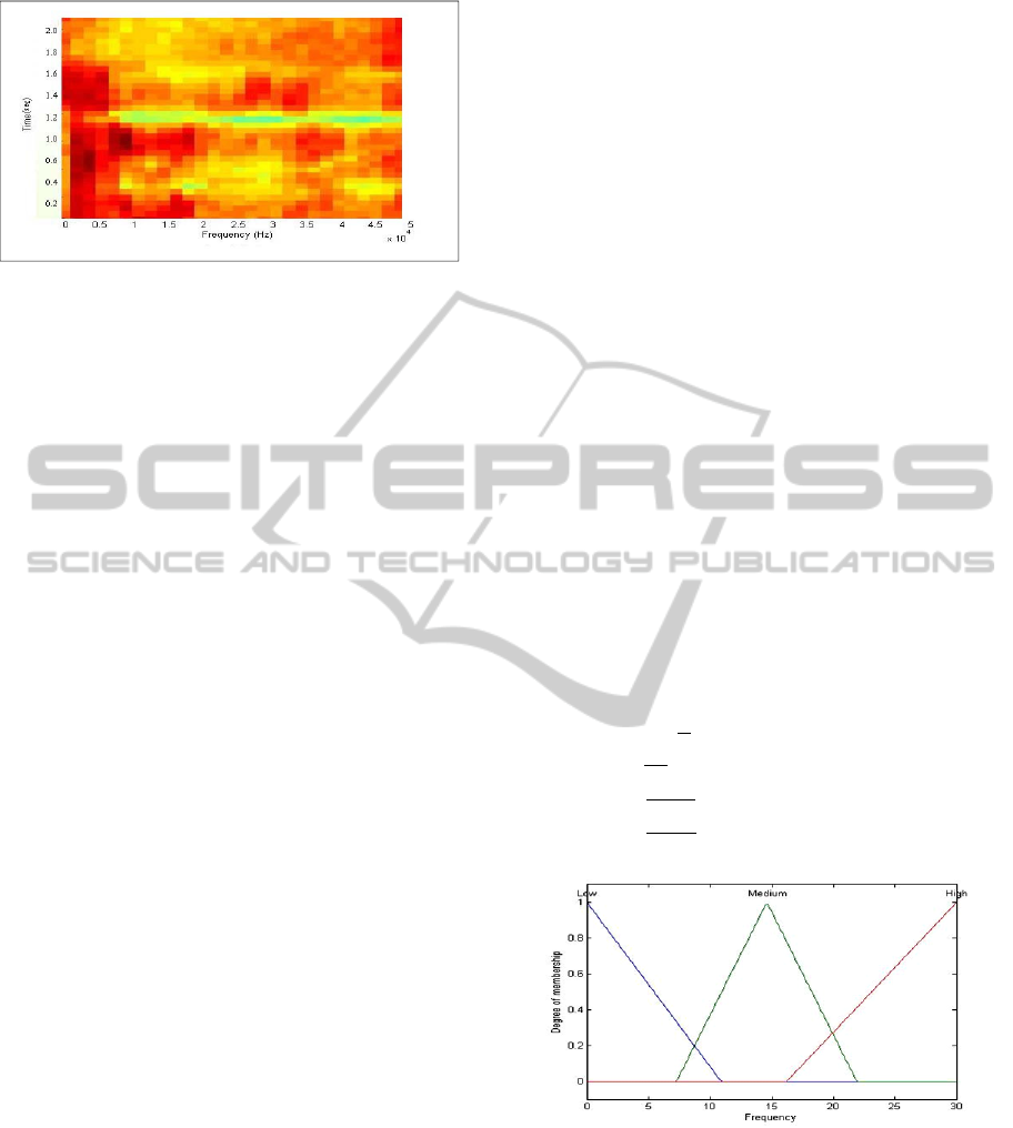
Figure 5: Spectrogram for the word “Bangladesh”
(downsampled to a 30 x 40 matrix).
Since we know that the human ear is more
sensitive to lower frequencies and vice versa for
higher frequencies, it would be wiser to divide the
frequency domain into exponentially growing
windows but instead of putting emphasize on the
lower frequencies, we decided to put more weight on
the overall evaluation on lower frequencies using
our Fuzzy Inference System (FIS).
3.5 Storing and/or altering Word
Descriptions
By downsampling the matrix is reduced to size
30 x 40. For each word, these matrices are stored in
our database along with a “Bengali” string that
represents the word speech in text. Altering a word
description is vividly described in subsection 3.7.
3.6 Comparison
The comparison is the base or ground of the fuzzy
logic implemented in our system. Before providing
details of FIS we need to mention the following facts
about our Fuzzy Inference System (FIS):
• We have 2 matrices, one for the sample (the
word to be recognised) and the other is the
target (the description of a word with which
it will be compared).
• The similarity of those two will be
determined by the closeness of their energy
values.
• The similarities will be prioritized by their
frequencies.
Next we present the details of the comparison
step:
1) The Comparison FIS membership functions:
In FIS, we have 3 inputs, i.e., frequency, target and
sample. Based on the inputs, the FIS will evaluate
the similarity of 2 segments and give us a result
ranging in the range [0, 10] where 10 being the
perfect match and 0 means no match (Figure 10).
The membership values are illustrated in the
following figures (Figure 6-8) and equations (eq. 6-
8). In Figure 6 the x axis represents 30 equal and
increasing segments of frequencies and the y axis
represents the degree of membership. To further
illustrate Figure 7 it is necessary to mention that all
the elements of the downsampled (subsection 3.4)
spectrogram – the 30 x 40 matrix of a word
description is normalized (ranging from 0 to 1). And
such energy values derived from the
STFT/Spectrogram are represented in the x axis of
both Figure 7 and Figure 8. In Figure 7, the x axis
represents the energy level (every element of the 30
x 40 matrix of a word description) of a particular
word in our database (which we are calling “target”).
On the other hand, the x axis of Figure 8 represents
the normalized energy level of a word spoken by a
user (which we are calling “sample”) which will be
compared to “target” as explained above. These
energy levels are also merely the elements of the 30
x 40 matrix generated through “downsampling”
(subsection 3.4) from the original spectrogram/STFT
(subsection 3.3) of the voiced data. In both Figure 7
and Figure 8, the y axis represents the degree of
membership.
µ
frequency
(x) =
+ 1, 0 11
, 6 15
, 15 22
+1, 16 30
(6)
Figure 6: Membership Function for Frequency
corresponding to equation (6).
BANGLA ISOLATED WORD SPEECH RECOGNITION
77
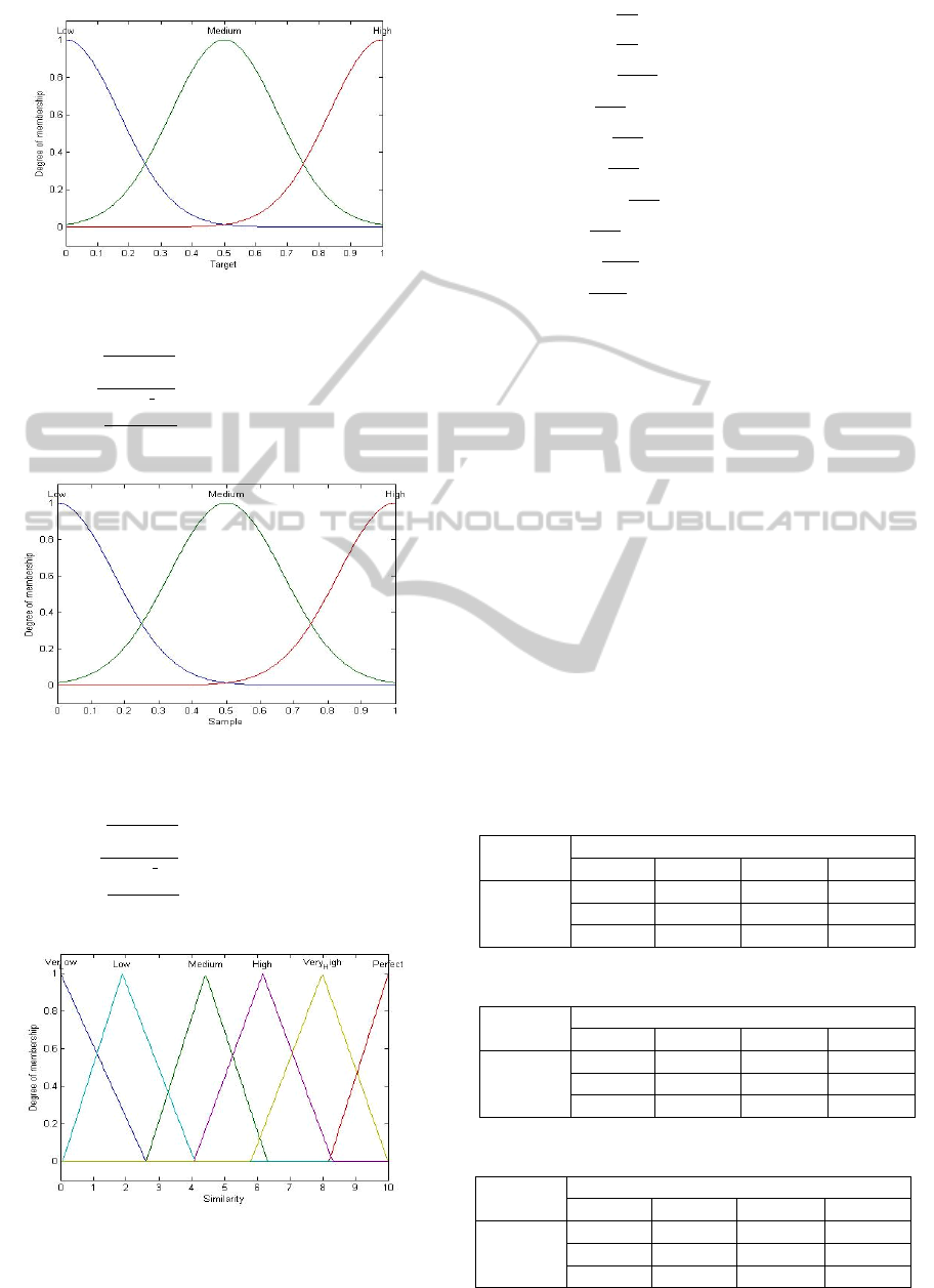
Figure 7: Membership Function for Target (energy level)
corresponding to equation (7).
µ
target
(x) =
.
, 0 0.5
.
.
, 0 1
.
,0.5 1
(7)
Figure 8: Membership Function for Sample (energy level)
corresponding to equation (8).
µ
sample
(x) =
.
, 0 0.5
.
.
, 0 1
.
,0.5 1
(8)
Figure 9: Membership Function for Output – Similarity,
corresponding to equation (9).
µ
similarity
(x) =
,03
+1,0 2
, 2 4
+ 1 ,2 4
,4 6
+ 1 ,4 6
,6 8
+ 1 ,6 8
,8 10
+1,810
(9)
The membership functions used in our systems
have been based on our sole understanding of the
recognition of speech. However the membership
function for “frequency” (equation 6 and Figure 6)
has been in accordance with the conventional model
of MEL spaced filterbanks (IIFP, 2010) even though
it has been modified as illustrated in Figure 6. All
the other membership functions (sample, target and
similarity) were derived from the visual
representation of the membership function shapes
(modelled by ourselves using MATLAB) based on
logical perception.
2) The fuzzy if-then rules: As we have 3 inputs,
we slice the three dimensional table into three two
dimensional tables (Table 1-3). Since we have 3
input variables, we use 27 or (2
3
) fuzzy propositions
(fuzzy if/then rules) to model our system. Also two
surface plots evaluating the model are presented in
Figure 10 and Figure 11.
Table 1: Fuzzy rules when frequency is LOW.
Sample
L
sam
p
le
M
sam
p
le
H
sam
p
le
Target
L
t
a
r
g
et
P M L
M
t
a
r
g
et
M P M
H
t
a
r
g
et
L M P
Table 2: Fuzzy rules when frequency is Medium.
Sample
L
sam
p
le
M
sam
p
le
H
sam
p
le
Target
L
t
a
r
g
et
VH M L
M
t
a
r
g
et
M VH M
H
t
a
r
g
et
VL M VH
Table 3: Fuzzy rules when frequency is high.
Sample
L
sam
p
le
M
sam
p
le
H
sam
p
le
Target
L
t
a
r
g
et
H M L
M
t
a
r
g
et
M H M
H
t
a
r
g
et
L M H
ICEIS 2011 - 13th International Conference on Enterprise Information Systems
78
The meanings of the terms in tables are given
below:
VL = Very Low
L = Low
M = Medium
H = High
VH = Very High
P = Perfect
From the rules it can be inferred that the lower
frequencies has been given higher priority when
evaluating the rules.
To get the complete view of the evaluation of the
FIS, Figure 10 and Figure 11 has been generated
using MATLAB. These two figures show the
evaluation of the aggregate of all the 27 fuzzy
propositions (if/then rules presented in Table 1, 2
and 3) and the membership functions shown in
Figure 6-8 as a surface plot. Since we have 3 input
variables (Frequency, Sample and Target) and 1
output variable (Similarity), the total number of
variables is 4 which cannot be accommodated in a
single figure (as four dimensions cannot be
represented in 3 dimensional form). Thus, we are
using 2 figures to illustrate the overall evaluation of
the FIS.
In Figure 10, the frequency (ranging from 0 to 30
as defined in the membership function in Figure 6) is
represented in the x axis. Here the variable “Sample”
is the word description (energy values of the 30 x 40
matrix) that the speaker has spoken which the
system identifies. Since it is normalized it is ranging
from 0 to 1 (Figure 8 shows the membership
function). Finally the similarity (ranging from 0 to
10 – based on our modelling as represented in fig 9)
is represented in the Z axis as output.
Figure 10: Surface illustrating the evaluation of the FIS
representing Frequency (X axis), Sample (Y axis) and
similarity (Z axis).
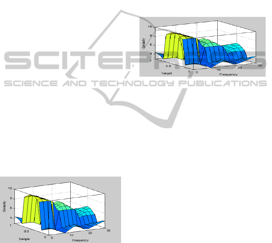
But Figure 10 cannot independently shed light on
the overall evaluation of the FIS. For that we need to
look at Figure 11 as well. Here the X axis and Z axis
are same as Figure 10 (frequency and similarity,
respectively). However, the Y axis is now “Target”
which is the word description (energy values of the
30 x 40 matrix) to which the “Sample” matrix is
compared. By “Target” we refer to a particular word
description (for a particular comparison) in our data-
set in form of a 30 x 40 matrix. Since it is
normalized, it is ranging from 0 to 1 (Figure 7 shows
the membership function). It is important to note that
the “Target” word description changes to the next
word in the data-set every time a particular
comparison of a word in the dataset (which we are
calling “Target”) to “Sample” (the word spoken by a
speaker) is computed.
Figure 11: Surface illustrating the evaluation of the FIS
representing Frequency (X axis), Target (Y axis) and
similarity (Z axis).
Now if we look at the surface plots of Figure 10
and Figure 11 then we notice that both the surfaces
are similar. It is because both “Sample” and
“Target” are normalized and they are reflected on
the similarity fuzzy propositions (Table 1-3).
Moreover, for achieving accurate similarity between
“Sample” and “Target” the membership functions
for both (equation. 7 and equation. 8 respectively)
are modelled as identical. In other words, if we
picture the two figures together then the similarity
will reach towards 10 (Figure 9 for membership
function plot) if “Sample” and “Target” have the
same or close values (based on the fuzzy if/then
rules).
It should be also noted that Figure 10 and Figure
11 conveys the fact that, lower frequencies are
getting higher priorities in the FIS than higher
frequencies. If we examine and go along the X axis
(which represents “Frequency”) then we see that the
height of the surface gradually decreases. This tells
us that as we move to higher frequencies from lower
ones, the similarity found between “Sample” and
“Target” are gradually given less weight in
“Similarity” which coincides to the fuzzy if/then
rules represented in Tables 1-3. For instance, if an
energy value of a particular segment (one particular
value in the 30 x 40 matrix of Sample) matches
completely with the energy value of the segment of
the same location of the “Target” (which is another
BANGLA ISOLATED WORD SPEECH RECOGNITION
79

30 x 40 matrix) then the similarity will not always
be 10. According to Figure 10 and Figure 11, if this
match is found when frequency value is one (every
frequency value corresponds to 167 Hz rising up to 5
KHz as discussed in Subsection 3.4) then the
similarity is given as ~ 9.9 on a scale of 10 (paying
more priority to lower frequencies), however if this
same matching takes place where frequency value is
25 (which corresponds to 25 x 167Hz = 4175 Hz as
mentioned in Subsection 3.4) then the similarity
value (defuzzified) is ~ 6.5 (on a scale of 10).
3.7 Training
After we feed our system with 50 words descriptions
(in form of 30 x 40 fuzzy sets), the user gets the
liberty to alter the description based on his/her
particular voice/tone/stress etc.
If a particular word – spoken by the user is
recognized incorrectly, then the system asks for the
correct word from the user (the user then types in
which word he/she has just spoken if and only if the
system fails to recognize the word itself). After
getting the inputs (voiced signal – which, in turn will
be converted into a 30 x 40 matrix as discussed in
Subsection 3.4, and the correct word string) – the
system compares this user’s input (voiced data that
has been converted into a 30 x 40 matrix as
explained in subsection 3.4) with the description of
our database. Based on the difference of the two, the
description stored in our database is altered in
accordance with the users speaking. Consequently,
the incorrect description will shift towards the user’s
version of the word.
To clarify the process let us consider that a user
has spoken a word that the system has recognized
incorrectly (suppose, user said the Bangla word
“Ek” but the system recognized it as the Bangla
word “Aat”). In that case the user prompts the
system that the match was incorrect and this
information is stored in a “Boolean” variable to
designate if the sample was a match or not. If it was
not a match (the system recognized the word
incorrectly) then the word description of the original
word will be altered as follows:
E
level(new)
= (E
level(original)
*original_weight)
+ (E
level(training)
* training_weight)
(10)
Here,
E
level(new)
= the energy level of a particular
segment of the spectrogram (every element of the 30
x 40 matrix of the word description and for this
example it is the description for the word “Ek”)
E
level(original)
= The energy level that was stored in
the database for the word that was spoken (or being
trained) by the user (and in this example the word is
“Ek”).
E
level(training)
= The energy level that the user had
just spoken which was identified incorrectly (and in
this example the word is “Ek”).
Original_weight = the weight of the energy level
of the original word description stored in the
database. We chose it to be
.
Training_weight = the weight of the energy level
of the word spoken by the user. We chose it to be
.
Therefore, we see that the summation of both the
weights gives us 1 (and whatever weight we choose
for modelling, the summation of the 2 weights has to
be 1), and from this we infer that the original word
description stored in the database will shift 50%
towards the word description of the word that a user
has just spoken.
On the other hand, the same system ends up
with different word descriptions with different
people, making it adaptive to the speaker’s voice.
Thus our system becomes user-adaptive with time.
Therefore the verdict can be reached that with time
our system develops more and more accuracy for a
particular user.
4 RESULT ANALYSIS
We have tested our system by categorizing words
into 3 categories. They are – mono-syllabic, bi-
syllabic and poly-syllabic. The total number of
Bangla words we tested for our system was 50 (20
of which were monosyllabic, 20 were bi-syllabic and
10 were polysyllabic).
By “mono-syllabic” we refer to the words that
have only one syllable i.e. Ek, dui, tin etc. (in
Bangla) or one, good, nice etc. (in English). Mono-
syllabic means the words that need only one stretch
of breath to pronounce. Then bi-syllabic are words
that need two stretches of breaths such as Kori (ko –
ri), Kathal (Ka – Thal), Kormo (kor – mo) etc. in
Bangla. Finally the polysyllabic words that we refer
to are words that have more than two syllables.
Example: prottutponnomotitto (prot-tut-pon-no-mo-
tit-to), Kingkortobbobimurho (king-kor-tob-bo-bi-
mur-ho) etc.
These are the criterions that have been kept as
constant in 5 different test case scenarios. In the
following subsections we analyse the accuracy of
ICEIS 2011 - 13th International Conference on Enterprise Information Systems
80
our system as follows: subsection 1 presents the
result when the system is trained by a male voice
and tested with a male voice and subsection 2
presents the results when the system is trained with
female voice and tested against a female voice.
Subsection 3, however presents the anomalous (non
adaptive) case where a female voice is tested when
the system has been trained by a male voice. A
similar scenario is presented in subsection 4 where a
male speaker was tested on a female-trained system.
Finally in subsection 5 we present the results of
accuracy when we compared our system against an
HMM based speech recognition software. In all the
scenarios the 50 Bangla words have been evaluated
as the data-set and the results are presented in regard
to monosyllabic, bi-syllabic and polysyllabic cases.
1) Male voice trained – Male speaker scenario: The
first test case scenario is the first and most general
analysis. Here the training was done by a male
speaker and the recognizing system was tested by a
different male speaker. It can be intuitively derived
that in this particular case the system gave one of the
most optimal accuracies. The comparison of the first
4 scenarios is presented in graphical form in Figure
12.
2) Female voice trained – Female speaker scenario:
This second scenario is similar to the scenario
presented in subsection 1. However, it has to be
noted that female voices reach higher frequencies for
a particular word than that of male speakers. The
natural average frequency of a male voice is 120 Hz
whereas for female voice it is 210 Hz (Traunmüller
and Eriksson, 1995). It will become more vivid in
subsection 3. Since in this scenario the training and
speaking, both have been done by a female speaker
(two different speakers but both female), the
accuracy reaches a relatively optimal level.
3) Male voice trained – Female speaker scenario:
In this scenario, the importance of training the
system becomes precise and illustrious. Intuitively
we may concur that if a speech recognition system
has been trained and optimized for male voice, it
will not perform as well as it would for whom it was
trained since the natural frequency range of females
are higher (~210Hz) than that of males (~210 Hz)
(Traunmüller and Eriksson, 1995). Our result
coincides with this fact.
It is self-explanatory that similar results are
achieved when the system has been trained using a
female voice and speaker happened to be a male.
The findings of this particular subsection and the
next one are important to realize the importance of
“training” and “user-adaptiveness” for speech
recognition systems.
4) Female voice trained – Male speaker scenario:
This scenario corresponds to the same test case as
described in subsection 3. Due to the mismatch of
frequencies, the system becomes less “speaker
adaptive” and the accuracy deters considerably. The
findings are presented in tabular form.
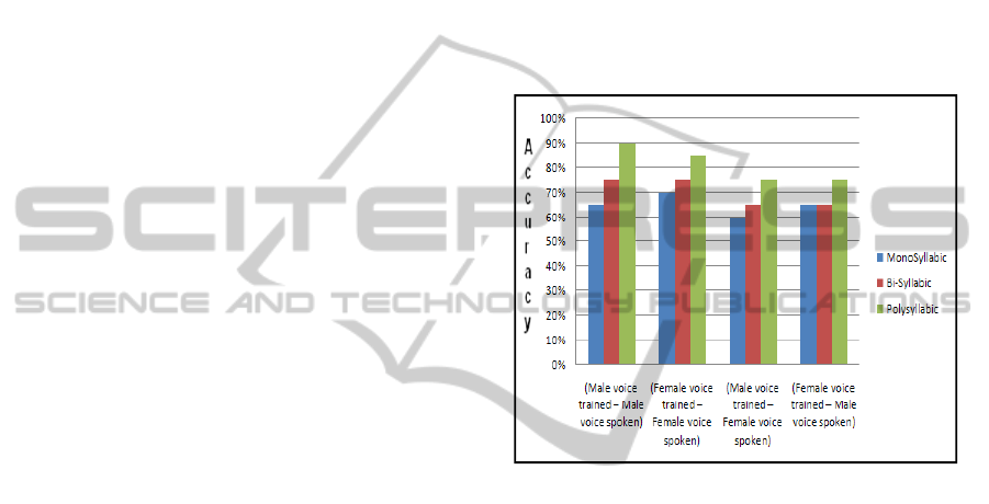
From the Figure 12 we can see that the findings
are similar to that of the findings analysed in
subsection 3. The aggregation of the findings of
subsection 1, 2, 3 and 4 are illustrated in Figure 12.
Figure 12: Aggregation of result analysis of subsections 1,
2, 3 and 4.
From the findings of subsection 1, 2, 3, 4 and
more appropriately Figure 12, it is clear that the
more appropriate training the system gets from the
speaker, the more user-adaptive it becomes and the
accuracy gets higher through training. The accuracy
rates presented in the paper are the accuracy rates at
the time of writing the paper; however, with more
training the accuracy rates, can, theoretically, get
higher (getting closer to 100% by every
incrementing training phase) drastically for a
particular speaker.
5) Comparison of our system against an HMM
based speech recognition system:
We had put our system against an HMM based
(phonetic level) speech recognition software –
Dragon Naturally Speaking (DNS, 2010) developed
by Nuance Communications (NComm, 2010). Since
the commercially developed software is phonetic
based it was language independent, giving us the
liberty to test it against our system but that software
gave us transliterations of Bengali words in English
rather than UNICODE Bangla text. The accuracy
BANGLA ISOLATED WORD SPEECH RECOGNITION
81
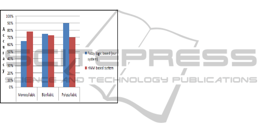
rates that we found are illustrated below in Figure
13.
It is an interesting finding that the fuzzy logic
based recognition recognizes the relatively more
difficult words (polysyllabic) better than HMM
systems to a greater extent than that of easier or
shorter words. It also coincides to our understanding
that our system gives better performance in Bangla
speech since it has been specifically trained for
Bangla word recognition and it works on the “word-
level” rather than the “phonetic level.”
Figure 13: Comparative result of HMM and Fuzzy logic
based system.
5 CONCLUSIONS
The system developed by us is one of the first
speech recognition attempts in Bangla speech using
fuzzy logic. However it is not without its limitations.
This particular system could be extended to
recognize continuous speech. Moreover the overall
accuracy of the system could be further improved
using the modern technical tools of today (even
though fuzzy logic has to be the base for all
linguistic ambiguity-related problems). As an end-
note it can be said that speech recognition was an
“open” problem before our system and it remains the
same upon completion of the system – but it is a
considerable step in reaching one of the solutions to
an “open” problem using spectral analysis and fuzzy
logic in Bangla speech.
REFERENCES
Abul, Md. H., Jabir, M., Mumit, K, 2007. Isolated and
Continuous Bangla Speech Recognition:
Implementation, Performance and application
perspective, in SNLP 07, Kasetsart University,
Bangok, Thailand
Davies, K. H., Biddulph, R., Balashek, S., 1952.
Automatic Speech Recognition of Spoken Digits, J.
Acoust. Soc. Am. 24(6) pp.637 –642.
Dragon Natural Speaking (DNS), 2010, Wikipedia
Encyclopedia, 2010. Available:
http://en.wikipedia.org/wiki/Dragon_NaturallySpeakin
g
Fletcher, H., 1922. The Nature of Speech and its
Interpretations, Bell Syst. Tech. J., Vol 1, pp. 129-
144.
Hasan, M. R., Nath, B., Alauddin B. M. , 2003. Bengali
Phoneme Recognition: A New Approach, in 6th ICCIT
conference, Dhaka.
Illinois Image Formation and Processing (IIFP), 2010.
DSP Mini-Project: An Automatic Speaker Recognition
System [Online]. Available:
http://www.ifp.illinois.edu/~minhdo/teaching/speaker_
recognition/speaker_recognition.html
Islam, M. R., Sohail, A. S. M., Sadid, M. W. H.M.,
Mottalib, A., 2005. Bangla Speech Recognition using
three layer Back-Propagation Neural Network, in
NCCPB, Dhaka.
Juang, B. H., Rabiner, L. R., 2005. Automatic Speech
Recognition -A Brief History of the Technology,
Elsevier Encyclopedia of Language and Linguistics,
Second Edition, Amsterdam, Holland.
Karim, A H M. R, Rahman, Md. S., Iqbal, Md.Zafar,
2002. Recognition of Spoken Letters in Bangla, in 6th
ICCIT conference, Dhaka.
Nuance Communications (NComm), (2010) Available:
http://www.nuance.com/naturallyspeaking/
Rahman, K. J., Hossain,M.A., Das, D., Islam, T. A. Z. and
Ali, M.G., 2003. Continuous Bangla Speech
Recognition System, in 6th Int. Conf. on Computer and
Information Technology (ICCIT), Dhaka.
Roy, K., Das, D., Ali, M.G, 2002. Development of the
Speech Recognition System Using Artificial Neural
Network, in 5th ICCIT conference, Dhaka.
Spectrogram on Wikipedia Encyclopedia, 2010. [Online].
Available: http://en.wikipedia.org/wiki/Spectrogram
Short-time Fourier Transform (STFT),Wikipedia
Encyclopedia, 2010. [Online]. Available:
http://en.wikipedia.org/wiki/STFT
Traunmüller, H., Eriksson, A., 1995. Publications of
Hartmut Traunmüller, Stockholm University, Sweden
[Online]. Available:
http://www.ling.su.se/staff/hartmut/f0_m&f.pdf
Weiss, M., 2006 . Indo-European Language and Culture,
Journal of the American Oriental Society [Online] .
Available:
http://findarticles.com/p/articles/mi_go2081/is_2_126/
ai_n29428508/
ICEIS 2011 - 13th International Conference on Enterprise Information Systems
82
