
COMPARISON OF SURFACE DATA
Exploring Real Samples Similarity for the Modelling of Engraving
Jana Hájková and Jakub Kotásek
Department of Computer Science and Engineering, University of West Bohemia, Univerzitní 8, Pilsen, Czech Republic
Keywords: Ablation, Laser engraving, Comparison, Real data, Confocal microscope, Similarity, MSE, PSNR.
Abstract: The paper deals with the topic of real samples comparison. The whole research is processed as a part of the
laser engraving modelling and simulation, for which real engraved and scanned samples are used as the
input and which are further processed before their usage. All samples are represented as height maps, so we
try to use MSE or PSNR computation for the comparison of samples. However, because of a special
character of the samples, several problems have to be solved. Finally, the results for the whole set of data
engraved into steel surface is presented and some interesting results are shown.
1 INTRODUCTION
This work is a part of larger project dealing with
development of a special laser device with precise
control and its modelling and simulation, which
should assure exact results usable for physical
research. All methods and results described in this
paper solve only a small but very important part of
the whole research of data pre-processing, more
concretely, the mutual comparison of processed real
samples.
Methods for sample comparison can be used for
example for the verification of the modelling and
simulation or, as shown in this paper, for exploring
real data. Real data comparison is important for
discovering the similarities among real samples and
the interaction between the laser beam and the
material surface. Because all the used methods are
already described in detail in (Hájková, 2008), only
some basics are outlined in Section 4, the main aim
of the paper is to show similarities and divergences
of real samples in dependence on the engraved
experiment (described in Section 5).
2 LASER ABLATION
Because we want to explore real samples and
compare them, we should first understand the
process of laser engraving and especially the
material ablation in detail. A laser beam is an
electromagnetic radiation. When this radiation
strikes a surface of a material, some radiation is
reflected, some absorbed and some transmitted. The
irradiated material is most affected by the absorbed
part of the radiation, which causes heating of the
surface. The heat generated in the surface directly
affected by the laser beam is conducted into the
material. If the laser intensity is high enough, the
material heats, melts, and if it reaches the boiling
point, it starts to vaporize. A part of vaporized
particles interacts with the laser beam and creates
plasma, the other particles, which are not affected by
the laser beam, approximately 18% of them as
mentioned in (Anisimov, 1968), condense back to
the surface of the material.
The previous description relates to the situation
when the laser irradiates the sample continuously
and the material is heated constantly during the
whole engraving. If we engrave more laser beam
pulses into one place on the surface, the temperature
of the material increases during each laser pulse.
Between each two consecutive pulses, the material
surface cools down in part, but not fully. That is why
the initial temperature is always higher and higher
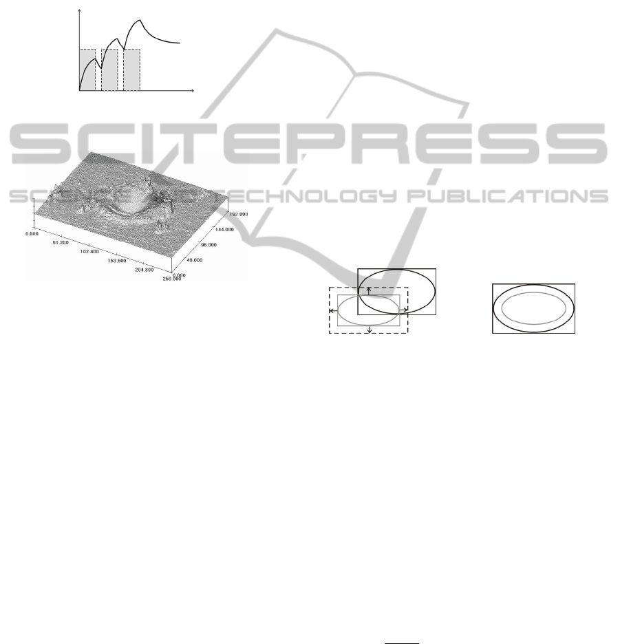
with each subsequent pulse. The evolution of
temperature of such sample is shown in Figure 1.
To sum up the whole engraving process: if the
surface of the material is exposed to an intense
pulsed laser beam it creates a rapid rise in local
temperature. The surface warms up and the material
starts to ablate. The ablated material then redeposites
around the irradiated area and together with various
273
Hájková J. and Kotásek J..
COMPARISON OF SURFACE DATA - Exploring Real Samples Similarity for the Modelling of Engraving.
DOI: 10.5220/0003485802730276
In Proceedings of the 6th International Conference on Software and Database Technologies (ICSOFT-2011), pages 273-276
ISBN: 978-989-8425-77-5
Copyright
c
2011 SCITEPRESS (Science and Technology Publications, Lda.)
local defects and original roughness of the material
causes many problems in samples processing.
Finally, at the exposure site, a pit with a transition
ring around it is left behind (an example can be seen
in Figure 2). The result of the engraving process
depends on the used material, its roughness, and
parameters of the laser. The whole process is
described in detail in (Dahotre and Harimkar, 2008)
or (Steen, 1991).
Figure 1: Evolution of surface temperature during
engraving multiple laser beam pulses into the same point.
Figure 2: Sample 3D view from the conf. microscope.
3 REAL DATA DESCRIPTION
As already mentioned, we use real data as the input
for the modelling of laser engraving. Samples
originate from real samples engraved by a laser into
a material surface. All samples are engraved into the
specified material (we use steel) with the given laser
(BLS-100 Nd:YAG solid-material, lamp-pumped
laser with the wavelength of 1064nm), each sample
is separately measured by a confocal microscope
(Olympus LEXT OLS3100) and saved in the form
of a height map. This height map is formed by a
matrix of real numbers, which express the heights in
a uniform rectangular grid. The dimensions of the
samples reach approximately several hundreds of
micrometers.
3.1 Experiment Description
We use the special testing data set consisting of
samples engraved by the laser into a single point of
the material. Such testing data should prevent
potential faults caused by the external influences in a
maximum possible way. The number of pulses goes
in sequence: 1, 2, 5, 10, 20, 30, ..., 100. Because
each sample is unique, samples differ from each
others even if the same experiment description has
been engraved repeatedly under the same conditions
and with the same laser settings. That is why each
experiment is repeated five times in order to get
sufficiently representative data set.
4 METHODS FOR COMPARISON
If we compare two height maps, we should make
sure that both the surfaces are aligned properly. That
is why it is very important to regularize all the
samples before the comparison itself. Moreover, we
need to compare only those areas which were
modified by the laser beam. For this purpose, we use
methods designed for the automatic detection of the
heat-affected area described, e.g. in (Hájková, 2011).
As can be seen in Figure 3a, the size of both
areas can differ and so we have to unify (enlarge)
the detected areas so that they both have the same
dimension and the heat-affected areas lie exactly in
the middle (as shown in Figure 3b).
a) b)
Figure 3: a) Two heat-affected areas of different sizes;
b) unifying expansion of selection dimensions.
Finally, the level of material in both the samples
is recomputed to have the same height. Then, we can
compute the similarity of both samples. For our test,
we have used two approaches: MSE and PSNR
computation described in following sections.
4.1 MSE (Mean Square Error)
This method computes the mean square error (MSE)
of two height maps. It is defined by the equation 1,
where W×H represent the dimensions of the height
maps and A(i, j) and B(i, j) indicate single points in
the given position [i,j] in the height map grid. The
resulting value expresses the average error for each
point.
() ()()
∑∑
−
=
−
=
−
×
=
1
0
1
0
2
,,
1
W
i
H
j
jiBjiA
HW
MSE
(1)
It is not difficult to see that the more identical the
samples are, the lower the MSE is computed. So, if
T
t
ICSOFT 2011 - 6th International Conference on Software and Data Technologies
274

we want to find a pair of height maps that are the
most similar, we look for the minimal value of MSE.
4.2 PSNR (Peak Signal-to-Noise Ratio)
The PSNR method uses MSE as a semi result. The
PSNR value is computed according to the equation
2, where the MAX value represents the highest point
in the height map.
⎟
⎟
⎠
⎞
⎜
⎜
⎝
⎛
=
MSE
MAX
PSNR
2
10
log.10
(2)
PSNR works in an inverse way, so if we are
looking for the most similar height maps, their
PSNR has to be the highest one.
5 RESULTS
We have used the approaches and methods described
above to explore a real data set to discover the
similarities and differences of samples. For our
testing, we have used an experiment described in
Section 3.1 that is a sequence of 1 to 100 laser beam
pulses engraved into a single point on a steel
surface. This sequence was engraved five times,
scanned and the heat-affected area was detected for
each sample.
In the next step, all samples were mutually
compared (each with each other) and the results of
MSE and PSNR were collected in (Kotásek, 2010).
Then we have selected different combinations of
comparisons and we were searching for variations
within them. Although there were some small
differences, the global trend was the same for all of
them and is discussed as follows. All values are
summarized in Table 1 (MSE) and Table 2 (PSNR).
5.1 Measured Values
Let us have a look on Table 1 first, where MSE
values are summarized. The more similar both tested
samples are, the smaller the MSE is computed. That
is why the smallest values are expected on the
diagonal of the table, where samples with the same
number of laser beam pulses are compared. In each
column of the table, the smallest value is highlighted
in bold. Although in some cases the minimal value
does not lie exactly on the diagonal, it is always very
close, most usually the neighbouring one. These
imperfections are typically caused by the local
defects that can be found in the samples. In Table 2
with PSNR results, the highest values are computed
for the most similar samples and are also highlighted
in bold. Also in this case similar problems with the
position of the maximal values can be found.
Besides exploring the real samples discussed in
Table 1: Results of the MSE computation.
1 2 5 10 20 30 40 50 60 70 80 90 100
1
0
,
69
2
,
00 1
,
55 11
,
89 12
,
51 10
,
90 9
,
66 27
,
27 29
,
13 41
,
58 44
,
87 23
,
80 44
,
38
2 2,00
1,35
3,26 10,81 11,55 10,37 8,98 24,55 26,41 37,52 40,83 21,41 40,33
5 1,55 3,26
0,81
10,73 11,59 9,91 9,70 27,24 29,40 42,41 45,73 24,91 45,27
10 11,89 10,81 10,73
1,16 2,10 2,50
2,34 7,04 9,41 16,04 18,69 8,04 17,67
20 12,51 11,55 11,59 2,10 2,37 3,01 2,56 7,27 9,53 16,43 18,82 8,37 18,40
30 10,90 10,37 9,91 2,50 3,01 2,83 2,75 8,65 10,80 18,30 20,68 9,19 20,34
40 9,66 8,98 9,70 2,34 2,34 2,75
1,15
6,99 8,78 16,00 18,22 6,70 19,15
50 27,27 24,55 27,24 7,04 7,27 8,65 6,99
2,40 4,23
6,23 8,04 3,79 7,70
60 29,13 26,41 29,40 9,41 9,53 10,80 8,78 4,23 5,07 7,06 8,69 4,33 8,73
70 41,58 37,52 42,41 16,04 16,43 18,30 16,00 6,23 7,06
5,04 6,85
6,12 6,23
80 44,87 40,83 45,73 18,69 18,82 20,68 18,22 8,04 8,69 6,85 7,19 7,67 7,85
90 23,80 21,41 24,91 8,04 8,37 9,19 6,70 3,79 4,33 6,12 7,67
1,03
7,72
100 44,38 40,33 45,27 17,67 18,40 20,34 19,15 7,70 8,73 6,23 7,85 7,72
3,45
Table 2: Results of the PSNR computation.
1 2 5 10 20 30 40 50 60 70 80 90 100
1
39
,
58
35
,
25 36
,
62 25
,
85 23
,
75 26
,
39 25
,
55 22
,
05 21
,
40 20
,
87 19
,
33 20
,
88 18
,
66
2 35,25
37,91
31,37 26,60 24,2 26,55 26,05 23,01 22,20 21,83 20,18 21,83 19,53
5 36,62 31,37
41,25
26,66 24,42 27,09 25,27 21,93 21,30 20,60 19,04 20,37 18,43
10 25,85 26,60 26,66
44,97 41,76 41,01
40,03 34,14 31,27 29,78 27,35 30,49 26,92
20 23,75 24,20 24,42 41,76 38,59 39,96 38,64 34,46 31,64 29,90 27,46 30,21 26,92
30 26,39 26,55 27,09 41,01 39,96 40,07 39,75 32,53 30,45 28,74 26,71 29,76 25,95
40 25,55 26,05 25,27 40,03 38,64 39,75
43,19
34,37 31,97 30,04 28,22 32,10s 26,18
50 22,05 23,01 21,93 34,14 34,46 32,53 34,37
42,51 40,61
39,07 35,60 39,62 34,78
60 21,40 22,20 21,30 31,27 31,64 30,45 31,97 40,61 39,18 39,55 36,54 38,88 34,51
70 20,87 21,83 20,60 29,78 29,90 28,74 30,04 39,07 39,55
40,86 39,21
40,20 38,25
80 19,33 20,18 19,04 27,35 27,46 26,71 28,22 35,60 36,54 39,21 37,09 36,86 35,93
90 20,88 21,83 20,37 30,49 30,21 29,76 32,10 39,62 38,88 40,20 36,86
47,32
34,44
100 18,66 19,53 18,43 26,92 26,92 25,95 26,18 34,78 34,51 38,25 35,93 34,44
40,71
COMPARISON OF SURFACE DATA - Exploring Real Samples Similarity for the Modelling of Engraving
275
this paper, we also wanted to discover, which
computational method is better to use for the
automatic determining of the most similar samples.
It is noticeable that the MSE and the PSNR give
analogous results for determining the similarity
(extremes in both tables are bold at the same
positions), but the MSE seems to give better results
for the automatic comparison, because the values
representing the most similar samples can be well
distinguished from the others (e.g. by thresholding).
The most similar samples are in Table 1 highlighted
with gray colour.
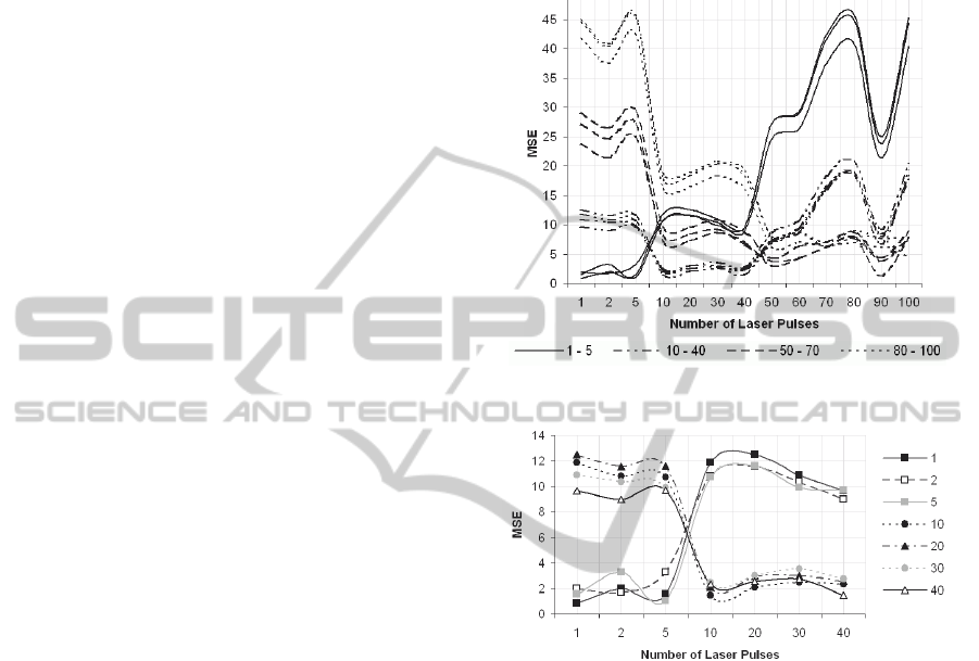
5.2 Results Visualization Discussion
Visualization of Table 1 brings some more
interesting facts. The MSE results can be seen in
Figure 4. In the plot, the horizontal axis shows the
sequence of samples and the curves express the
similarity of the individual samples. The distance
between the samples determined as similar and not-
similar is noticeable. An interesting characteristic
can be seen in the plot the cumulating of the curves
representing the similarity of a sample to each other.
If we take a look more closely, we can see that
curves representing the samples with small number
of pulses (1, 2 and 5) are placed close to each other
in the plot. Also, the values in Table 1 do not differ a
lot. The same situation can be discovered for
samples with 10 to 40 pulses and then for samples
with 50 to 100 pulses. So, samples can be divided
into groups, in which they are similar to each other,
but are very different from samples in the other
groups. This is also the reason, why the curves are
not labelled separately, but only in sets. The
situation between two groups is more closely shown
in Figure 5.
6 CONCLUSIONS
As can be seen from the described results and plots,
the number of laser pulses engraved into one point
of the material influences the ablation process a lot.
What is the reason of the described relations?
Accumulating temperature during the ablation
process and so changing nature of the irradiated
material. The heated material behaves differently if
it is heated for a while or for a longer time.
So far, we have studied mainly samples engraved
into steel, where all the laser pulses were engraved
into a single point on the material surface. Our
further plan is to explore the results when the laser is
moving above the material surface with a constant or
even a variable speed. In our future work, we would
also like to conduct more experiments with different
laser settings and/or engraved into different
materials and search for the next dependencies, how
the engraved experiments influence the ablation
process and the final shape of the material surface.
Figure 4: MSE results visualization.
Figure 5: MSE computation results – detail of sweeping
change of samples similarity.
REFERENCES
Anisimov, S. I., 1968: Vaporization of metal absorbing
laser radiation. Soviet Physics JETP, Vol. 27, pp. 182.
Dahotre, N. B., Harimkar, S. P., 2008: Laser Fabrication
and Machining of Materials, Springer, New York,
USA.
Hájková, J., 2008: Approaches for Automatic Comparison
of Laser Burned Samples, Proceedings of the 9
th
International PhD Workshop on Systems and Control.
Izola, Slovenia.
Hájková, J., 2011: Laser Engraving Modelling: Compari-
son of Methods for the Heat-Affected Area Detection,
Proceedings of the 10
th
International Conference
APLIMAT 2011. STU Bratislava, Slovakia.
Kotásek, J.: Metody porovnávání výškových map (Methods
for Height Maps Comparison), Bachelor Thesis,
University of West Bohemia, 2010.
Steen, W. M., 1991: Laser Material Processing.
Springer-Verlag, New York Berlin Heidelberg.
ICSOFT 2011 - 6th International Conference on Software and Data Technologies
276
