
RESOURCE-AWARE HIGH QUALITY CLUSTERING
IN UBIQUITOUS DATA STREAMS
Ching-Ming Chao
Department of Computer Science and Information Management, Soochow University, Chinese Taiwan
Guan-Lin Chao
Department of Electrical Engineering, National Taiwan University, Chinese Taiwan
Keywords: Data Mining, Data Streams, Clustering, Ubiquitous Data Mining, Ubiquitous Data Stream Mining.
Abstract: Data stream mining has attracted much research attention from the data mining community. With the ad-
vance of wireless networks and mobile devices, the concept of ubiquitous data mining has been proposed.
However, mobile devices are resource-constrained, which makes data stream mining a greater challenge. In
this paper, we propose the RA-HCluster algorithm that can be used in mobile devices for clustering stream
data. It adapts algorithm settings and compresses stream data based on currently available resources, so that
mobile devices can continue with clustering at acceptable accuracy even under low memory resources. Ex-
perimental results show that not only is RA-HCluster more accurate than RA-VFKM, it is able to maintain a
low and stable memory usage.
1 INTRODUCTION
Due to rapid progress of information technology, the
amount of data is growing very fast. How to identify
useful information from these data is very important.
Data mining is to discover useful knowledge from
large amounts of data. Data generated by many ap-
plications are scattered and time-sensitive. If not
analyzed immediately, these data will soon lose their
value; e.g., stock analysis and vehicle collision pre-
vention (Kargupta et al., 2002; Kargupta et al.,
2004). How to discover interesting patterns via mo-
bile devices anytime and anywhere and respond to
the user in real time faces major challenges, result-
ing in the concept of ubiquitous data mining (UDM).
With the advance of sensor devices, many data
are transmitted in the form of streams. Data streams
are large in amount and potentially infinite, real
time, rapidly changing, and unpredictable (Babcock
et al., 2002; Golab and Ozsu, 2003). Compared with
traditional data mining, ubiquitous data mining is
more resource-constrained, such as constrained
computing power and memory size. Therefore, it
may result in mining failures when data streams
arrive rapidly. Ubiquitous data stream mining thus
has become one of the newest research topics in data
mining.
Previous research on ubiquitous data stream clus-
tering mainly adopts the AOG (Algorithm Output
Granularity) approach (Gaber et al., 2004a), which
reduces output granularity by merging clusters, so
that the algorithm can adapt to available resources.
Although the AOG approach can continue with
mining under a resource-constrained environment, it
sacrifices the accuracy of mining results. In this
paper, we propose the RA-HCluster (Resource-
Aware High Quality Clustering) algorithm that can
be used in mobile devices for clustering stream data.
It adapts algorithm settings and compresses stream
data based on currently available resources, so that
mobile devices can continue with clustering at ac-
ceptable accuracy even under low memory re-
sources.
The rest of this paper is organized as follows.
Section 2 reviews related work. Section 3 presents
the RA-HCluster algorithm. Section 4 shows our
experimental results. Section 5 concludes this paper
and suggests some directions for future research.
64
Chao C. and Chao G..
RESOURCE-AWARE HIGH QUALITY CLUSTERING IN UBIQUITOUS DATA STREAMS.
DOI: 10.5220/0003467700640073
In Proceedings of the 13th International Conference on Enterprise Information Systems (ICEIS-2011), pages 64-73
ISBN: 978-989-8425-53-9
Copyright
c
2011 SCITEPRESS (Science and Technology Publications, Lda.)
2 RELATED WORK
Aggarwal et al. (2003) proposed the CluStream
clustering framework that consists of two compo-
nents. The online component stores summary statis-
tics of the data stream. The offline component uses
summary statistics and user requirements as input,
and utilizes an approach that combines micro-
clustering with pyramidal time frame to clustering.
The issue of ubiquitous data stream mining was
first proposed by Gaber et al. (2004b). They ana-
lyzed problems and potential applications arising
from mining stream data in mobile devices and pro-
posed the LWC algorithm, which is an AOG-based
clustering algorithm. LWC performs adaptation
process at the output end and adapts the minimum
distance threshold between a data point and a cluster
center based on currently available resources. When
memory is full, it outputs the merged clusters.
Shah et al. (2005) proposed the RA-VFKM algo-
rithm, which borrows the effective stream clustering
technique from the VFKM algorithm and utilizes the
AOG resource-aware technique to solve the problem
of mining failure with constrained resources in
VFKM. When the available memory reaches a criti-
cal stage, it increases the value of allowable error
(ε*) and the value of probability for the allowable
error (δ*) to decrease the number of runs and the
number of samples. Its strategy of increasing the
value of error and probability compromises on the
accuracy of the final results, but enables conver-
gence and avoids execution failure in critical situa-
tions.
The RA-Cluster algorithm proposed by Gaber
and Yu (2006) extends the idea of CluStream and
adapts algorithm settings based on currently avail-
able resources. It is the first threshold-based micro-
clustering algorithm and it adapts to available re-
sources by adapting its output granularity.
3 RA-HCLUSTER
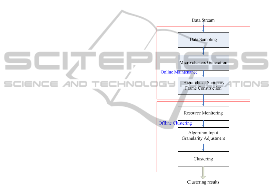
As shown in Figure 1, RA-HCluster consists of two
components: online maintenance and offline cluster-
ing. In the online maintenance component, summary
statistics of stream data are computed and stored,
and then are used for mining by the offline cluster-
ing component, thereby reducing the computational
complexity. First, the sliding window model is used
to sample stream data. Next, summary statistics of
the data in the sliding window are computed to gen-
erate micro-clusters, and summary statistics are
updated incrementally. In addition, the calculation of
correlation coefficients is included in the process of
merging micro-clusters to improve the problem of
declining accuracy caused by merging micro-
clusters. Finally, a hierarchical summary frame is
used to store cluster feature vectors of micro-
clusters. The level of the hierarchical summary
frame can be adjusted based on the resources avail-
able. If resources are insufficient, the amount of data
to be processed can be reduced by adjusting the
hierarchical summary frame to a higher level, so as
to reduce resource consumption.
Figure 1: RA-HCluster.
In the offline clustering component, algorithm
settings are adapted based on currently available
memory, and summary statistics stored in the hierar-
chical summary frame are used for clustering. First,
the resource monitoring module computes the usage
and remaining rate of memory and decides whether
memory is sufficient. When memory is low, the size
of the sliding window and the level of the hierarchi-
cal summary frame are adjusted using the AIG (Al-
gorithm Input Granularity) approach. Finally, clus-
tering is conducted. When memory is low, the dis-
tance threshold is decreased to reduce the amount of
data to be processed. Conversely, when memory is
sufficient, the distance threshold is increased to
improve the accuracy of clustering results.
RESOURCE-AWARE HIGH QUALITY CLUSTERING IN UBIQUITOUS DATA STREAMS
65
3.1 Online Maintenance
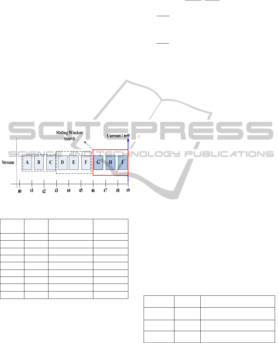
3.1.1 Data Sampling
The sliding window model is used for data stream
sampling. Figure 2 shows an example of sliding
window sampling, in which Stream represents a data
stream and t
0
, t
1
, …, t
9
each represents a time point.
Suppose the window size is set to 3, which means
three data points from the stream are extracted each
time. Thus, the sliding window first extracts three
data points A, B, and C at time points t
1
, t
2
,
and t
3
,
respectively. After the data points within the win-
dow are processed, the window moves to the right to
extract the next three data points. In this example,
the window moved a total of three times and ex-
tracted a total of nine data points at time points from
t
1
to t
9
. Table 1 shows the sampled stream data.
Figure 2: Example of sliding window sampling.
Table 1: Sampled stream data.
Data
point
Age Salary
(in thousands)
Arrival
timestamp
A 36 34 t1
B 30 21 t2
C 44 38 t3
D 24 26 t4
E 35 27 t5
F 35 31 t6
G 48 40 t7
H 21 30 t8
I 50 44 t9
3.1.2 Micro-cluster Generation
For sampled data points, we use the K-Means algo-
rithm to generate micro-clusters. Each micro-cluster
is made up of n d-dimensional data points
n
xx ...
1
and their arrival timestamp
n
tt ...
1
. Next, we
compute summary statistics of data points of each
micro-cluster to obtain its cluster feature vector,
which consists of
)32(
+
× d
data entries and is
represented as (
x
CF 2
,
x
CF 1
,
t
CF 2
,
t
CF 1
,
n
).
Data entries are defined as follows:
x
CF 2
is the squared sum of dimensions, and
the squared sum of the e
th
dimension can be ex-
pressed as
2
1
)(
∑
=
n
j
e
j
x
.
x
CF1
is the sum of dimensions, and the sum of
the e
th
dimension can be expressed as
∑
=
n
j
e
j
x
1
.
t
CF 2
is the squared sum of timestamp
n
tt ...
1
,
and can be expressed as
∑
=
n
j
j
t
1
2
.
t
CF1
is the sum of timestamp
n
tt ...
1
, and can
be expressed as
∑
=
n
j
j
t
1
.
n
is the number of data points
The following are the steps for generating micro-
clusters:
Step 1: Compute the mean of sampled data.
Step 2: Compute the square distance between the
mean and each data point, and find the data point
nearest to the mean as a center point. Then move the
window once to extract data.
Step 3: If the current number of center points is
equal to the user-defined number of micro-clusters
q, execute Step 4; otherwise, return to Step 1.
Step 4: Use the K-Means algorithm to generate q
micro-clusters with q center points as cluster cen-
troids, and compute the summary statistics of data
points of each micro-cluster.
Assume that the user-defined number of micro-
clusters is three. Table 2 shows the micro-clusters
generated from the data points of Table 1, in which
the micro-cluster Q
1
contains three data points B
(30, 21), D (24, 26), and H (21, 30) and the cluster
feature vector is computed as {(
2
30
+
2
24
+
2
21
,
2
21
+
2
26
+
2
30 ), (30+24+21, 21+26+30),
2
2
+
2
4
+
2
8
, 2+4+8, 3} = {(1917,2017), (75,77), 84,
14, 3}.
Table 2: Micro-clusters generated.
Micro-cluster Data points Cluster feature vector
Q
1
B, D, H ((1917,2017), (75,77), 84, 14, 3)
Q
2
A, E, F ((3746,2846), (106,92), 62, 12, 3)
Q
3
C, G, I ((6740,4980), (142,122), 139, 19, 3)
Next, we set a maximum radius boundary
λ
.
When a new data point p arrives at the data stream,
if the square distance
),(
2
i
mpd
between p and its
nearest micro-cluster center m
i
is less than
λ
, p is
ICEIS 2011 - 13th International Conference on Enterprise Information Systems
66
()
1
1
k
ii
i
k
k
i
i
W
W
β
β
β
=
=
⎛⎞
×
⎜⎟
⎝⎠
=
⎛⎞
⎜⎟
⎝⎠
∑
∑
merged into micro-cluster M
i
; otherwise, a new
micro-cluster is generated for p. When the current
number of micro-clusters is greater than the user-
defined number, two of the micro-clusters must be
merged. In the merge process, we not only compute
the distance similarity between micro-clusters, but
also use Pearson correlation coefficient
γ
to identify
the two most similar micro-clusters to merge in
order to improve the problem of reduced accuracy
caused by merge. Equation (1) is the calculation
formula for Pearson correlation coefficient and is
used for computing the direction and level of change
of data points for each micro-cluster. The value
of
γ
is between -1 and 1. A greater
γ
means a greater
level of change; that is, the degree of correlation
between two micro-clusters is greater.
(1)
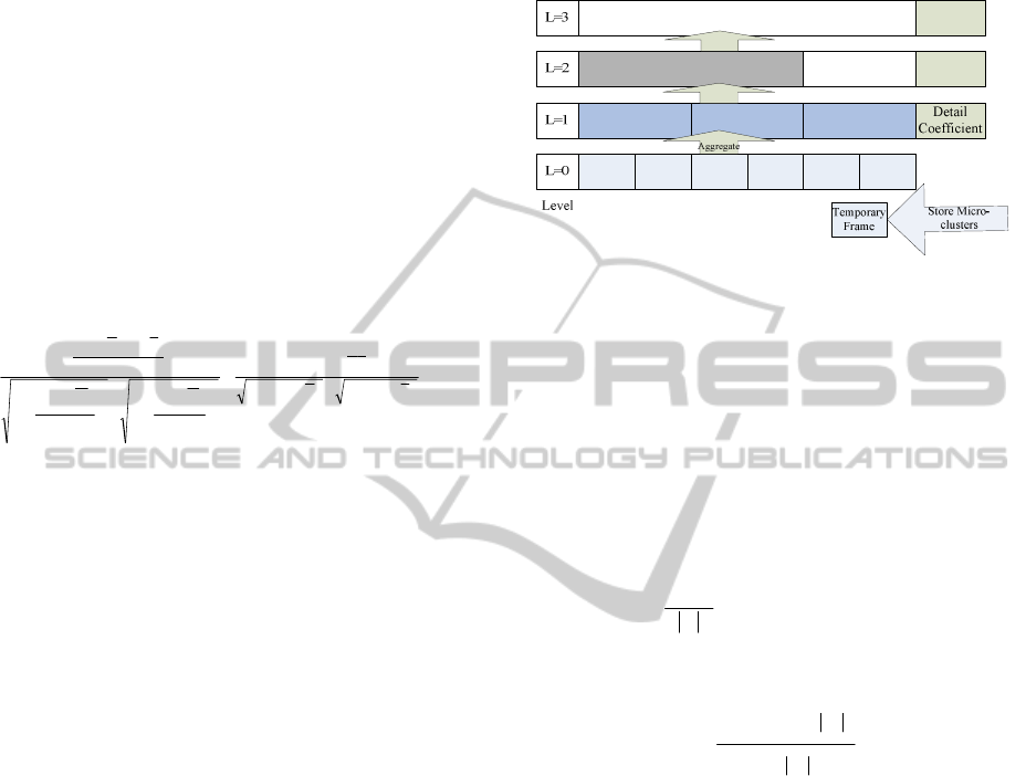
3.1.3 Hierarchical Summary Frame
Construction
After micro-clusters are generated, we propose the
use of a hierarchical summary frame to store cluster
feature vectors of micro-clusters and construct level
0 (L = 0), which is the current level, of the hierarchi-
cal summary frame. In the offline clustering compo-
nent, the cluster feature vectors stored at the current
level of the hierarchical summary frame will be used
as virtual points for clustering. In addition, the hier-
archical summary frame is equipped with two func-
tions: data aggregation and data resolution. When
memory is low, it performs data aggregation to ag-
gregate detailed data of lower level into summarized
data of upper level to reduce the consumption of
memory space and computation time for clustering.
But if there is sufficient memory, it will perform
data resolution to resolve summarized data of upper
level back to detailed data of lower level.
The representation of the hierarchical summary
frame is shown in Figure 3.
L
is used to indicate a level of the hierarchical
summary frame. Each level is composed of
multiple frames and each frame stores the clus-
ter feature vector of one micro-cluster.
Each frame can be expressed as
[
]
es
j
i
ttF ,
, in
which
s
t is the starting timestamp,
e
t is the end-
ing timestamp, and i and j are the level number
and frame number, respectively.
A detail coefficient field is added to each level
above level 0 of the hierarchical summary
frame, which stores the difference of data and
is used for subsequent data resolution.
],[
0
1
0 t
ttF
],[
21
2
0 tt
ttF
+
],[
312
3
0 tt
ttF
+
],[
20
1
1 t
ttF
],[
412
2
1 tt
ttF
+
],[
614
3
1 tt
ttF
+
],[
413
4
0 tt
ttF
+
],[
514
5
0 tt
ttF
+
],[
615
6
0 tt
ttF
+
],[
40
1
2 t
ttF
Figure 3: Hierarchical summary frame.
The process of data aggregation and data resolu-
tion utilizes the Haar wavelet transform, which is a
data compression method characterized by fast cal-
culation and easy understanding and is widely used
in the field of data mining (Dai et al., 2006). This
transform can be regarded a series of mean and dif-
ference calculations. The calculation formula is as
follows:
The use of wavelet transform to aggregate
frames in the interval can be expressed as
()
β
β
β
∑
=
=
1i
i
F
W
, in which F represents the
frame.
k wavelet transforms can be expressed as
(2)
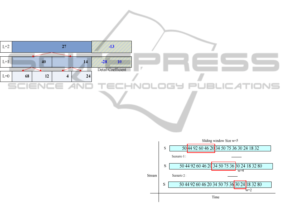
Figure 4 shows an example of hierarchical sum-
mary frame, in which the aggregation interval
β
is
set to 2, indicating that two frames are aggregated in
each data aggregation process. Suppose the current
level L = 0 stores four micro-clusters, and the sums
of dimension are 68, 12, 4, and 24, respectively,
represented as
}24,4,12,68{
0
=
L
. When memory is
low, data aggregation is performed. Because the
aggregation interval is 2, it first computes the aver-
age and difference of the first frame
1
0
F
and the sec-
ond frame
2
0
F
of level 0, resulting in the value
(12+68)/2=40
and detail coefficient (12-68)/2=-28
of the first frame
1
1
F
of level 1, and then derives the
timestamp
[
]
3,0
of
1
1
F
by storing the starting time-
stamp of
1
0
F
and the ending timestamp of
2
0
F
. It then
moves on to the third frame
3
0
F
and the fourth
()()
() ()
∑∑
∑
∑
−
−
∑
−
−
∑
−×−
−
=
⎟
⎟
⎠
⎞
⎜
⎜
⎝
⎛
×
⎟
⎟
⎠
⎞
⎜
⎜
⎝
⎛
−
−−
2222
22
11
1
YnYXnX
YXnXY
n
YYXX
n
YY
n
XX
RESOURCE-AWARE HIGH QUALITY CLUSTERING IN UBIQUITOUS DATA STREAMS
67
frame
4
0
F
of level 0, resulting in the value
(24+4)/2=14, detail coefficient (24-4)/2=10, and
timestamp
[]
7,4
of the second frame
2
1
F
of level 1.
After all frames of level 0 are aggregated, the data
aggregation process ends and level 1 of the hierar-
chical summary frame is constructed, which is rep-
resented as
}14,40{
1
=L
. Other levels of the hier-
archical summary frame are constructed in the same
way. In addition, we can obtain the Haar transform
function
(
)
(
)
(
)
10,28,13,27 −−=xfH
by storing the
value and detail coefficient of the highest level of
the hierarchical summary frame, which can be used
to convert the aggregated data back to the data be-
fore aggregation.
]1,0[
1
0
F
]3,0[
1
1
F
]7,0[
1
2
F
]3,2[
2
0
F
]5,4[
3
0
F
]7,6[
4
0
F
]7,4[
2
1
F
)10,28,13,27())(( −
−
=xfH
Figure 4: Example of hierarchical summary frame.
When there is sufficient memory, data resolution
is performed to convert the aggregated data back to
the detailed data of lower level, using the Haar trans-
form function obtained during data aggregation. To
illustrate, assume that the current level of the hierar-
chical summary frame is
L=2.
}14,40{
1
=L
is ob-
tained by performing subtraction and addition on the
value and detail coefficient of level 2, {40,
14}={[27-(-13), 27+(-13)]}.
L
0
= {68, 12, 4, 24} is
obtained in the same way, except that there are two
values and detail coefficients at level 1. Therefore,
to obtain {68, 12, 4, 24} = {[40-(-28), 40+(-28), 14-
10, 14+10]}, we first perform subtraction and addi-
tion on the first value and detail coefficient, then
perform the same calculation on the second value
and detail coefficient.
3.2 Offline Clustering
3.2.1 Resource Monitoring and Algorithm
Input Granularity Adjustment
In the offline clustering component, we use the re-
source monitoring module to monitor memory. This
module has three parameters
m
N
,
m
U
, and
m
LB
,
which represent the total memory size, current
memory usage, and lowest boundary of memory
usage, respectively. In addition, we compute the
remaining rate of memory
mmmm
NUNR /)( −=
.
When
<
m
R
m
LB
, meaning that memory is low, we
will adjust the algorithm input granularity. Algo-
rithm input granularity adjustment refers to reducing
the detail level of input data of the algorithm in
order to reduce the resources consumed during algo-
rithm execution. Therefore, when memory is low,
we will adjust the size of the sliding window and the
level of the hierarchical summary frame in order to
reduce memory consumption.
First, we adjust the size of the sliding window. A
larger window size means a greater amount of
stream data to be processed, which will consume
more memory. Thus, we multiply the window size
w
by the remaining rate of memory
m
R
to obtain the
adjusted window size. As
m
R
gets smaller, so is the
window size.
Figure 5 shows an example of window
size adjustment, with the initial window size
w set to
5. In scenario 1, the memory usage
m
U
is 20 and the
computed
m
R
is 0.8. Then, through
58.0 ×=× wR
m
we obtain the new window size of 4, so we reduce
the window size from 5 to 4. In scenario 2, the
memory usage
m
U
is 60 and the computed
m
R
is 0.4.
Then, through
54.0 ×
=
×
wR
m
we obtain the new
window size of 2, so we reduce the window size
from 5 to 2.
458.0,8.0
100
20100
,20,100 =×==
−
=== wRUN
mmm
254.0,4.0
100
60100
,60,100 =×==
−
=== wRUN
mmm
Figure 5: Example of window size adjustment.
Next, we perform data aggregation to adjust the
level of the hierarchical summary frame. This proc-
ess will be done only when
m
R
< 20% because it
will reduce the accuracy of clustering results. On the
other hand, we will perform data resolution when
(
)
m
R
−
1
< 20%, which indicates there is sufficient
memory. The process of data aggregation and data
resolution has been described in details in Section
3.1.3.
3.2.2 Clustering
Figure 6 shows the proposed clustering algorithm.
The algorithm inputs the number of clusters
k, the
ICEIS 2011 - 13th International Conference on Enterprise Information Systems
68
distance threshold
d
, the lowest boundary of mem-
ory usage
m
LB
, and the cluster feature vectors
stored in the current level of the hierarchical sum-
mary frame as virtual points
x. The algorithm out-
puts the finally generated
k clusters C. The steps of
the algorithm are divided into three parts. The first
part is for cluster generation (line 4-10). Every vir-
tual point is attributed to the nearest cluster center to
generate
k clusters. The second part is for the ad-
justment of distance threshold
d
(line 11-14). The
adjustment of
d
is based on the current remaining
rate of memory. A smaller
d
implies that virtual
points are more likely to be regarded as outliers and
discarded in order to reduce memory usage. The
third part is for determination of the stability of
clusters (line 15-31). Recalculate cluster centers of
the clusters generated in the first part and use the
sample variance and total deviation to determine the
stability of clusters. Output the clusters if they are
stable; otherwise repeat the process by returning to
the first part.
The parameters of the clustering algorithm are
defined as follows:
k is the user-defined number of clusters.
d
is the user-defined distance threshold.
m
LB
is the user-defined lowest boundary of
memory usage.
}1{ nixx
i
≤≤=
is the set of virtual points
stored in the current level of the hierarchical
summary frame.
}1{ kjCC
j
≤≤=
is the set of k clusters gener-
ated by the algorithm.
m
N
is the total memory size
}1{ kjcc
j
≤≤=
is the set of k cluster centers.
),(
2
ji
cxd
is the Euclidean distance between
virtual point
x
i
and cluster center c
j
.
}1,1),({
2
kjnicxdD
jii
≤≤≤≤=
is the set
of Euclidean distances between virtual point
x
i
and each cluster center, with the initial value
of ∅.
][
i
DMin
is the Euclidean distance between vir-
tual point
x
i
and its nearest cluster center.
m
U
is the memory usage.
m
R
is the remaining rate of memory.
E
is the total deviation.
2
S
is the sample variance.
)(
j
Ccount
is the number of virtual points in the
cluster
j
C
.
E
′ is the total deviation calculated from the new
cluster center.
2
ˆ
S
is the sample variance calculated from the
new cluster center.
Input: k,
d
,
m
LB
,
x
Output:
C
1.
compute
m
N
;
2.
←
c
Random (x);
3. Repeat
4. For each
xx
i
∈
do
5.
For each
cc
j
∈
do
6.
)},({
2
jiii
cxdDD ∪←
;
7.
If
][
i
DMin
<
d
then
8.
}{
ijj
xCC ∪←
s.t.
][),(
2
iji
DMincxd =
;
9.
Else
10.
delete
i
x
;
11. compute
m
U
;
12.
mmmm
NUNR /)(
−
←
;
13.
If
m
R
<
m
LB
then
()
m
Rddd −×−← 1
;
14.
If
(
)
m
R−1
<20%
then
×+← ddd
m
R
;
15.
For each
j
C
do
16.
∑
∈
−←
ji
Cx
ji
cxE
2
)(
;
17.
()( )
1)(/
2
2
−
⎟
⎟
⎠
⎞
⎜
⎜
⎝
⎛
−←
∑
∈
j
Cx
ji
CcountcxS
ji
;
18.
)(/)(
j
Cx
ij
Ccountxc
ji
∑
∈
←
′
;
19.
If
jj
cc
≠
′
then
20.
∑
∈
′
−←
′
ji
Cx
ji
cxE
2
)(
;
21.
()( )
1)(/
ˆ
2
2
−
⎟
⎟
⎠
⎞
⎜
⎜
⎝
⎛
′
−←
∑
∈
j
Cx
ji
CcountcxS
ji
;
22.
If (
2
ˆ
S
<
2
S
) and (
E
′
<
E
) then
23.
jj
cc
′
←
;
24.
Else
25. output
j
C
;
26.
ji
Cx
∈
∀
}{
i
xxx
−
←
;
27.
}{
j
ccc
−
←
;
28. Else
29.
output
j
C
;
30.
ji
Cx
∈
∀
}{
i
xxx
−
←
;
31.
}{
j
ccc
−
←
;
32.
Until
j
C
∀
)(
jj
cc
=
′
or
)
ˆ
(
22
SS ≥
or
)( EE ≥
′
33. return;
Figure 6: Clustering algorithm.
RESOURCE-AWARE HIGH QUALITY CLUSTERING IN UBIQUITOUS DATA STREAMS
69
The following is a detailed description of the
steps of the clustering algorithm.
Step 1 (line 1): Use a system built-in function to
compute the total memory size.
Step 2 (line 2): Use a random function to ran-
domly select
k virtual points as initial cluster centers.
Step 3 (line 4-10): For each virtual point, com-
pute the Euclidean distance between it and each
cluster center. If the Euclidean distance between a
virtual point and its nearest cluster center is less than
the distance threshold, the virtual point is attributed
to the cluster to which the nearest cluster center
belongs; otherwise, the virtual point is deleted.
Step 4 (line 11-14): Compute the memory us-
age
m
U
and the remaining rate of memory
m
R
. If
m
R
<
m
LB
, meaning that memory is low, then de-
crease
d
by subtracting the value of multiplying
d
by the memory usage rate
()
m
R−1
. When the
memory usage rate is higher,
d
is decreased more.
On the other hand, if
()
m
R−1
<20%, meaning that
memory is sufficient, then increase
d
by adding the
value of multiplying
d
by the remaining rate of
memory
m
R
. When the remaining rate of memory is
higher,
d
is increased more.
Step 5 (line 15-31): Steps 5.1 and 5.2 are exe-
cuted for each cluster.
Step 5.1 (line 16-18): Compute the sample vari-
ance
2
S
and the total deviation
E
of virtual points
contained in the cluster. Next, compute the mean of
virtual points contained in the cluster as the new
cluster center
j
c
′
.
Step 5.2 (line 19-31): If the new cluster cen-
ter
j
c
′
is the same as the old cluster center
j
c
, then
output the cluster
j
C
, meaning that
j
C
will not change
any more, and delete the virtual points and cluster
center of
j
C
; otherwise, use
j
c
′
to recalculate the
sample variance
2
ˆ
S
and the total deviation
E
′
, and
determine whether both
2
ˆ
S
and
E
′ are decreased. If
yes, replace the old cluster center with the new one;
otherwise, output the cluster
j
C
and delete the virtual
points and cluster center of
j
C
.
Repeat the execution of Step 3 to Step 5 until for
every cluster the cluster center is not changed or the
sample variance or total deviation is not decreased.
Assume k = 2,
d
= 10,
m
LB
= 30%, and the vir-
tual points stored in the current level of the hierar-
chical summary frame are A (2,4), B (3,2), C (4,3),
D (5,6), E (8,7), F (6,5), G (6,4), H (7,3), I (7,2), the
algorithm output two clusters
1
C
= [A, B, C] and
2
C
=
[D, F, G, H, I].
4 PERFORMANCE EVALUTION
4.1 Experimental Environment
and Data
To simulate the environment of mobile devices, we
use Sun Java J2ME Wireless Toolkit 2.5 as the de-
velopment tool to write programs and conduct per-
formance evaluation on the J2ME platform. Table 3
shows the experimental environment.
Table 3: Experimental environment.
Component Specification
Processor Pentium D 2.8 GHz
Memory 1 GB
Hard disk 80 GB
Operating system Windows XP
We use the ACM KDD-CUP 2007 consumer
recommendations data set as the real data set. This
data set contains 480,000 customer data, 17,000
movie data, and 1 million recommendations data
recorded between October 1998 and December
2005. We use 200,000 recommendations data for the
experiments. Furthermore, in order to use a variety
of number of data points and dimensions to carry out
the experiments, we use Microsoft SQL Server 2005
with Microsoft Visual Studio Team Edition for Da-
tabase Professional to generate synthetic data sets,
which are in uniform distribution. Table 4 shows the
description of generating parameters of synthetic
data. All data points are sampled evenly from C
clusters. All sampled data points show a normal
distribution. For example, B100kC10D5 represents
that this data set contains 100k data points belonging
to 10 different clusters and each data point has 5
dimensions.
Table 4: Generating parameters of synthetic data.
Parameter Description
B Number of data points
C Number of clusters
D Number of dimensions
4.2 Comparison and Analysis
As RA-VFKM is also a ubiquitous data stream clus-
tering algorithm that can continue with mining under
constrained resources, we compare the performance
between RA-HCluster and RA-VFKM in terms of
stream processing efficiency, accuracy, and memory
usage.
ICEIS 2011 - 13th International Conference on Enterprise Information Systems
70
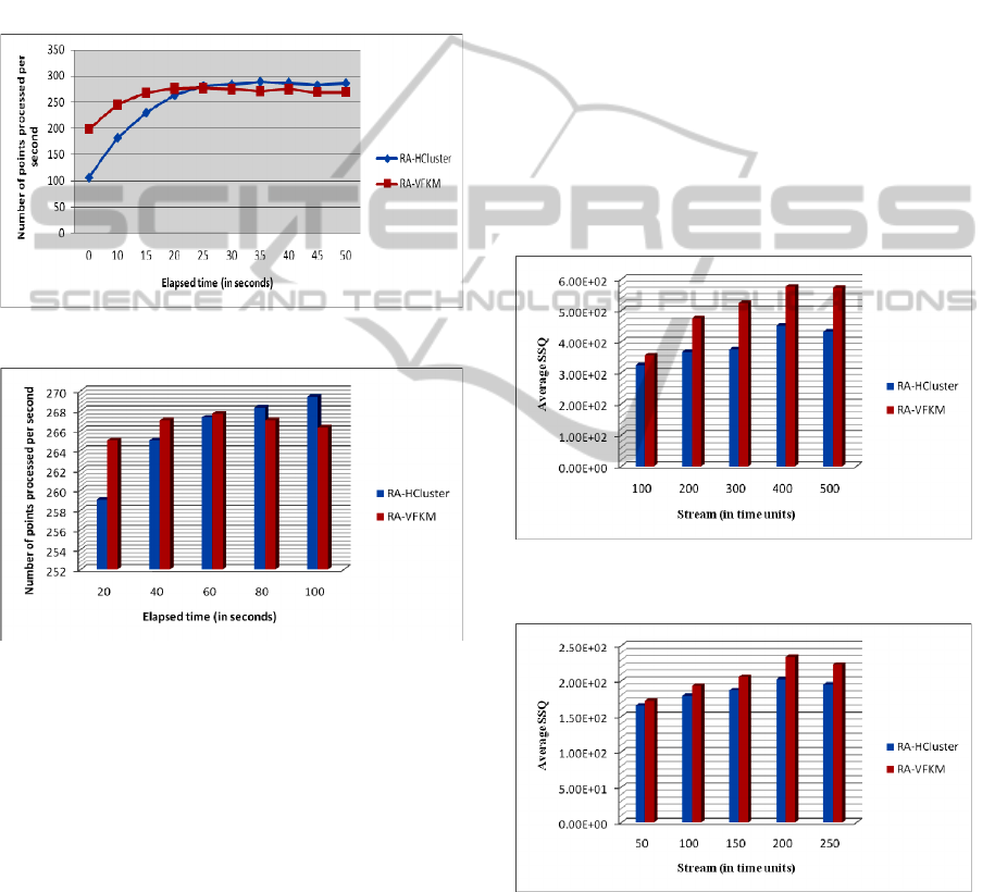
4.2.1 Stream Processing Efficiency
We use the number of data points processed per
second to measure the stream processing efficiency
with the consumer recommendations data set as
experimental data. Figure 7 and Figure 8 show the
comparison of stream processing efficiency between
RA-HCluster and RA-VFKM, where the horizontal
axis is the elapsed data processing time in seconds
and the vertical axis is the number of data points
processed per second.
Figure 7: Comparison of stream processing efficiency.
Figure 8: Comparison of stream processing efficiency for
a longer elapsed time.
As shown in Figure 7, because RA-HCluster
needs to generate micro-clusters and compute cluster
feature vectors as soon as stream data arrive, the
initial stream processing is more inefficient. After 20
seconds while micro-clusters have been generated,
the stream processing efficiency of RA-HCluster
increases and stabilizes. In contrast, because RA-
VFKM uses Hoeffding Bound to limit the sample
size, the initial stream processing efficiency is better.
But over time, the stream processing efficiency of
RA-VFKM is worse than that of RA-HCluster.
As shown in Figure 8, for a longer elapsed time,
the stream processing efficiency of RA-HCluster is
poor only initially. By the 60th second, its stream
processing efficiency is about the same as RA-
VFKM, and it gradually overtakes RA-VFKM in
terms of stream processing efficiency after 80 sec-
onds.
4.2.2 Accuracy
We use the average of the sum of square distance
(Average SSQ) to measure the accuracy of cluster-
ing results. Suppose there are
h
n
data points in the
period
h
before the current time T
c
. Find the nearest
cluster center
ni
c for each data point
h
n
in the period
h
and compute the square distance
),(
2
nii
cnd
be-
tween
i
n and
ni
c . The ),( hTSSQAverage
c
for the
period h before the current time T
c
equals to the sum
of all square distances between every data point in
h
and its cluster center divided by the number of clus-
ters. A smaller value of Average SSQ indicates a
higher accuracy.
Figure 9: Comparison of accuracy with consumer recom-
mendations data set.
Figure 10: Comparison of accuracy with synthetic data set.
Figure 9 and Figure 10 show the comparison of
accuracy between RA-HCluster and RA-VFKM
with the consumer recommendations data set and
synthetic data set, respectively. The horizontal axis
is the data rate (e.g., data rate 100 means that stream
data arrive at the rate of 100 data points per second)
RESOURCE-AWARE HIGH QUALITY CLUSTERING IN UBIQUITOUS DATA STREAMS
71
and the vertical axis is the Average SSQ. As shown
in Figure 9 and Figure 10, the accuracy of RA-
HCluster is about the same as that of RA-VFKM
only when the data rate is from 50 to 100. When the
data rate is over 200, the accuracy of RA-HCluster is
higher than that of RA-VFKM.
In Figure 10, the differences in Average SSQ are
not obvious because synthetic data of the same dis-
tribution are used, but we can still see that the Aver-
age SSQ of RA-HCluster is smaller. The reason is
that RA-HCluster uses the distance similarity be-
tween micro-clusters as the basis for merge, and
employs the sample variance to identify more dense
clusters in the offline clustering component, so as to
increase the clustering accuracy. In contrast, RA-
VFKM increases the error value
ε
to reduce the
sample size and merges clusters to achieve the goal
of continuous mining, so as to reduce the clustering
accuracy.
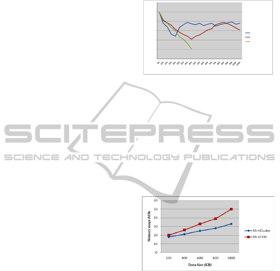
4.2.3 Memory Usage
Because the greatest challenge in mining data
streams using mobile devices lies in the constrained
memory of mobile devices and insufficient memory
may lead to mining interruption or failure, we com-
pare the capability of continuous mining of algo-
rithms by analyzing their memory usage. Figure 11
shows the comparison of memory usage among RA-
HCluster, RA-VFKM, and traditional K-Means,
where the horizontal axis is the elapsed data process-
ing time in seconds and the vertical axis is the re-
maining memory in megabytes (MB). The experi-
mental data is the consumer recommendations data
set, with a parameter setting of C = 10, data rate =
100, and
m
N
= 100 MB. As shown in Figure 11,
traditional K-Means is not able to continue with
mining and mining interruption occurs after 450
seconds. Although RA-VFKM is able to continue
with mining, it is incapable of adapting to the evolu-
tion of data stream effectively because the fluctua-
tion in memory usage is very large. In contrast, even
though RA-HCluster uses more memory in the be-
ginning, it is able to maintain low and stable mem-
ory usage thereafter. The reason is that RA-VFKM
releases resources by merging clusters at the end of
the clustering process, but RA-HCluster adapts algo-
rithm settings during the clustering process so that
mining can be stable and sustainable.
0
20
40
60
80
100
120
Remaining memory (MB)
Elapsed time (in seconds)
RA‐HClust e r
RA‐VFKM
traditionalK‐Means
Figure 11: Comparison of memory usage.
Figure 12 shows the comparison of memory us-
age between RA-HCluster and RA-VFKM under a
variety of data size, where the horizontal axis is the
data size in kilobytes (KB) and the vertical axis is
the memory usage in megabytes (MB). The experi-
mental data is the consumer recommendations data
set. As shown in Figure 12, RA-VFKM requires
more memory under various sizes of data and its
memory usage increases significantly when the data
size is over 600 KB. In contrast, because RA-
HCluster compresses data in the hierarchical sum-
mary frame through the data aggregation process, it
can still maintain a stable memory usage even when
dealing with larger amounts of data.
Figure 12: Comparison of memory usage by data size.
Figure 13 shows the comparison of memory us-
age between RA-HCluster and RA-VFKM under a
variety of execution time, where the horizontal axis
is the elapsed data processing time in seconds and
the vertical axis is the memory usage in megabytes
(MB). The experimental data is a synthetic data set
B100kC10D5. As shown in Figure 13, even though
RA-HCluster uses more memory in the beginning, it
then decreases the memory usage by reducing the
input granularity. After 40 seconds, therefore, the
memory usage is decreased and stabilized. In con-
trast, RA-VFKM uses less memory than RA-
HCluster only in the beginning, and it uses more
memory after 37 seconds.
ICEIS 2011 - 13th International Conference on Enterprise Information Systems
72
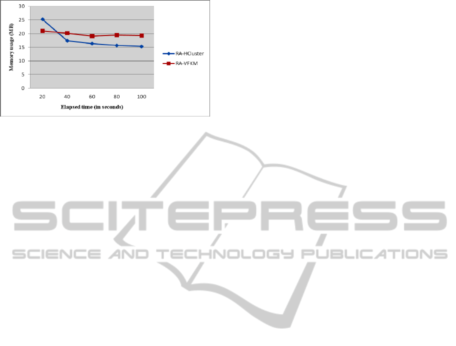
Figure 13: Comparison of memory usage by execution
time.
5 CONCLUSIONS AND FUTURE
WORK
In this paper, we have proposed the RA-HCluster
algorithm for ubiquitous data stream clustering. This
algorithm adopts the resources-aware technique to
adapt algorithm settings and the level of the hierar-
chical summary frame, which enables mobile de-
vices to continue with mining and overcomes the
problem of lower accuracy or mining interruption
caused by insufficient memory in traditional data
stream clustering algorithms. Furthermore, we in-
clude the technique of computing the correlation
coefficients between micro-clusters to ensure that
more related data points are attributed to the same
cluster during the clustering process, thereby im-
proving the accuracy of clustering results. Experi-
mental results show that not only is the accuracy of
RA-HCluster higher than that of RA-VFKM, it can
also maintain a low and stable memory usage.
Because we have only dealt with mining a single
data stream using mobile devices in this paper, for
future research we may consider dealing with multi-
ple data streams. In addition, we can consider factors
such as battery, CPU utilization, and data rate to the
resource-aware technique, so that algorithms can be
more effectively adapted with respect to the current
environment of mobile devices and the characteris-
tics of data stream. For practical applications, we
may consider applications such as vehicle collision
prevention, intrusion detection, stock analysis, etc.
ACKNOWLEDGEMENTS
The authors would like to express their appreciation
for the financial support from the National Science
Council of Republic of China under Project No.
NSC 99-2221-E-031-005.
REFERENCES
Aggarwal, C. C., Han, J., Wang, J., Yu, P. S., 2003. A
Framework for Clustering Evolving Data Streams. In
Proceedings of the 29th International Conference on
Very Large Data Bases, Berlin, Germany, pp. 81-92.
Babcock, B., Babu, S., Motwani, R., Widom, J., 2002.
Models and Issues in Data Stream Systems.
In Pro-
ceedings of the 21st ACM SIGMOD Symposium on
Principles of Database Systems
, Madison, Wisconsin,
U.S.A., pp. 1-16.
Dai, B. R., Huang, J. W., Yeh, M. Y., Chen, M. S., 2006.
Adaptive Clustering for Multiple Evolving Streams.
IEEE Transactions on Knowledge and Data Engineer-
ing, Vol. 18, No. 9, pp. 1166-1180.
Gaber, M. M., Zaslavsky, A., Krishnaswamy, S., 2004.
Towards an Adaptive Approach for Mining Data
Streams in Resource Constrained Environment.
In
proceedings of the International Conference on Data
Warehousing and Knowledge Discovery,
Zaragoza,
Spain, pp. 189-198.
Gaber, M. M., Krishnaswamy, S., Zaslavsky, A., 2004.
Ubiquitous Data Stream Mining. In
Proceedings of the
8th Pacific-Asia Conference on Knowledge Discovery
and Data Mining
, Sydney, Australia.
Gaber, M. M., Yu, P. S., 2006. A Framework for Re-
source-aware Knowledge Discovery in Data Streams:
A Holistic Approach with Its Application to Cluster-
ing. In
Proceedings of the 2006 ACM Symposium on
Applied Computing, Dijon, France, pp. 649-656.
Golab, L., Ozsu, T. M., 2003. Issues in Data Stream Man-
agement
ACM SIGMOD Record, Vol. 32, Issue 2, pp.
5-14.
Kargupta, H., Park, B. H., Pittie, S., Liu, L., Kushraj, D.,
Sarkar, K., 2002. MobiMine: Monitoring the Stock
Market from a PDA.
ACM SIGKDD Explorations
Newsletter, Vol. 3, No. 2, pp. 37-46.
Kargupta, H., Bhargava, R., Liu, K., Powers, M., Blair, P.,
Bushra, S., Dull, J., Sarkar, K., Klein, M., Vasa, M.,
Handy, D., 2004. VEDAS: a Mobile and Distributed
Data Stream Mining System for Real-Time Vehicle
Monitoring. In
Proceedings of the 4th SIAM Interna-
tional Conference on Data Mining, Florida, U.S.A.,
pp. 300-311.
Shah, R., Krishnaswamy, S., Gaber, M. M., 2005. Re-
source-Aware Very Fast K-Means for Ubiquitous Data
Stream Mining. In
Proceedings of 2nd International
Workshop on Knowledge Discovery in Data Streams
,
Porto, Portugal, pp. 40-50.
RESOURCE-AWARE HIGH QUALITY CLUSTERING IN UBIQUITOUS DATA STREAMS
73
