
BUILDING VISUAL MAPS WITH A SINGLE OMNIDIRECTIONAL
CAMERA
Arturo Gil, David Valiente, Oscar Reinoso, Lorenzo Fern´andez and J. M. Mar´ın
Departamento de Ingenier´ıa de Sistemas y Autom´atica, Miguel Hern´andez University
Avda. de la Universidad s/n, Alicante, Elche, Spain
Keywords:
SLAM, Visual SLAM, Omni-directional images.
Abstract:
This paper describes an approach to the Simultaneous Localization and Mapping (SLAM) problem using a
single omnidirectional camera. We consider that the robot is equipped with a catadioptric sensor and is able
to extract interest points from the images. In the approach, the map is represented by a set of omnidirectional
images and their positions. Each omnidirectional image has a set of interest points and visual descriptors
associated to it. When the robot captures an omnidirectional image it extracts interest points and finds corre-
spondences with the omnidirectional images stored in the map. If a sufficient number of points are matched, a
translation and rotation can be computed between the images, thus allowing the localization of the robot with
respect to the images in the map. Typically, visual SLAM approaches concentrate on the estimation of a set of
visual landmarks, each one defined by a 3D position and a visual descriptor. In contrast with these approaches,
the solution presented here simplifies the computation of the map and allows for a compact representation of
the environment. We present results obtained in a simulated environment that validate the SLAM approach.
In addition, we present results obtained using real data that demonstrate the validity of the proposed solution.
1 INTRODUCTION
Many applications in the field of mobile robots re-
quire the existence of a map that represents the en-
vironment. Thus, the construction of a map is a key
ability for an autonomous vehicle. In order to build
the map the robot must explore the environment to
gather data and compute a coherent map. Commonly,
the pose of the robot during the exploration process is
unknown, leading to the problem of Simultaneous Lo-
calization and Mapping (SLAM). In these situations,
the robot needs to build a map incrementally, while,
simultaneously, computes its location inside the map.
To date, due to their precision, laser range sensors
have been used to build maps (Stachniss et al., 2004;
Montemerlo et al., 2002). Typically, these applica-
tions use directly the laser measurements to build 2D
occupancy grid maps (Stachniss et al., 2004), or they
extract features from the laser measurements (Monte-
merlo et al., 2002) to build 2D landmark-based maps.
During the last years, a great number of ap-
proaches propose the utilisation of cameras as the
main sensor in SLAM. These applications are usually
denoted as visual SLAM. Compared to laser ranging
systems, cameras are typically less expensiveand pro-
vide a huge quantity of 3D information (projected on
a 2D image), whereas typical laser range systems al-
low to collect distance measurements only on a 2D
plane. However, vision sensors are generaly less pre-
cise than laser sensors and require a significant com-
putational effort in order to find usable information
for the SLAM process.
Different approaches to SLAM using vision sen-
sors have been classified under the name of visual
SLAM. In these group, we can find stereo-based ap-
proaches in which two calibrated cameras are used to
build a 3D map of the environment, which is repre-
sented by a set of visual landmarks referred to a com-
mon system, being each landmark accompanied by
a visual descriptor computed from its visual appear-
ance. Other approaches use a single camera to build
a map of the environment. For example in (Civera
et al., 2008) a single camera is used to build a 3D
map of the environment of visual landmarks extracted
with the Harris corner detector (Harris and Stephens,
1988). The camera is moved by hand. When viewed
from different viewpoints separated with a sufficient
baseline, the 3D position of the landmarks can be es-
timated. The trajectory of the camera and the position
145
Gil A., Valiente D., Reinoso O., Fernández L. and M. Marín J..
BUILDING VISUAL MAPS WITH A SINGLE OMNIDIRECTIONAL CAMERA.
DOI: 10.5220/0003459701450154
In Proceedings of the 8th International Conference on Informatics in Control, Automation and Robotics (ICINCO-2011), pages 145-154
ISBN: 978-989-8425-75-1
Copyright
c
2011 SCITEPRESS (Science and Technology Publications, Lda.)
of the landmarks can be estimated up to a scale factor.
The performance of the single-camera SLAM is im-
proved when using a wide field of view lens (Andrew
J. Davison et al., 2004), which suggests that using
an omni-directional camera would be advantageous
in visual SLAM, since the horizontal field of view is
maximum.
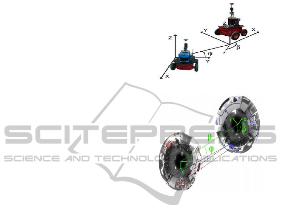
We consider the case in which a mobile robot is
equipped with a single omni-directional camera, as
shown in Figure 1(a). Each image is processed to ex-
tract interest points that can be matched from differ-
ent viewpoints. We consider that the robot captures
an omnidirectional image. Next, the robot moves and
captures a different omnidirectional image. If we as-
sume that a set of significant points can be extracted
and matched in both images, the relative movement
between the images can be computed (Scaramuzza
et al., 2009). In particular, the rotation between im-
ages can be univoquely computed, as well as the
translation (up to a scale factor). To obtain these
measurements between images we rely on a modifica-
tion of the Seven Point Algorithm (Scaramuzza et al.,
2009). In Figure 1(b) we present two omnidirectional
images, where some correspondences have been in-
dicated. The transformation between both reference
systems is shown. In the experiments we rely on the
SURF features for the detection and description of the
points. In the SLAM infrastructure presented here,
the image I
0
will be named a view, in order to differ-
entiate from the commonly used visual landmarks. In
this sense, a view is an image captured from a pose
in the environment that is associated with a set of bi-
dimensional points extracted from it. It is worth not-
ing that a visual landmark corresponds to a physical
point, such as a corner on a wall. However, the view
represents the visual information that is obtained from
a particular pose in the environment.
In this paper we propose a different representa-
tion of the environment in the visual SLAM problem.
Instead of estimating the position of a set of visual
landmarks in the environment we consider the posi-
tion and orientation of a set of views in the environ-
ment. When the robot moves in the neighbourhood of
the view and captures an image with the camera, a set
of interest points will be matched between the current
image and the view, thus allowing to localize the robot
with respect to it. When the robot moves away from
the image, the appearance of the scene will vary and it
may be difficult to find corresponding points. In this
case, a new view will be created at the currentposition
of the robot with an uncertainty. The new view will al-
low the localization of the robot around its neighbour-
hood. It is worth noting that this representation has
been previously used in the context of localization.
(a)
(b)
Figure 1: Figure 1(a) shows the sensor setup used during the
experiments. Figure 1(b) presents two real omnidirectional
images acquired, with some correspondences indicated.
For example, in (Fernandez et al., 2010) a set of om-
nidirectional images acquired at certain points in the
environment are used to localize the environment us-
ing a Monte-Carlo algorithm and a global appearance-
based comparison of the images. In (Konolige et al.,
2010) a view-based map is proposed. Connections
between different stereo views are formed by consis-
tent geometric matching of their features. The map is
estimated with a graph optimization technique. How-
ever, in the approach presented here, an omnidirec-
tional camera is used instead, which allows us to rep-
resent the environment with a low number of omni-
directional images. In addition, the transformation
between views can only be computed up to a scale
factor, thus the restrictions between views cannot be
geometric.
The approach proposed in this paper presents
some advantages over previous visual SLAM ap-
proaches. The most important is the compactness of
the representation of the environment. For example,
in (AndrewJ. Davison et al., 2004; Civera et al., 2008)
an Extended Kalman Filter (EKF) is used to estimate
ICINCO 2011 - 8th International Conference on Informatics in Control, Automation and Robotics
146

the position of the visual landmarks, as well as the po-
sition and orientation of the camera. In (Civera et al.,
2008) 6 variables are used to represent each landmark,
thus the state vector in the EKF grows rapidly with
the number of landmarks in the environment. This
fact poses a challenge for most existing SLAM ap-
proaches. In opposition with these, in the algorithm
presented here, only the pose of a reduced set of views
is estimated. Thus, each view encapsulates informa-
tion of a particular area in the environment, in the
form of several interest points detected in the image.
Typically, as will be shown in the experiments, a sin-
gle view may retain a sufficient number of interest
points so that the localization in its neighbourhood
can be performed.
The main disadvantage of the presented approach,
is, nevertheless, the computational cost of determin-
ing a metric transformation between two omnidirec-
tional images. However, in Section 4 we present an
algorithm that can be used to process images at a fast
rate and can be used for online SLAM. In this case,
the computation of the transformation between two
images depends only on the number of matches, that
can be easily adjusted to provide both speed and pre-
cise results.
We present a series of results obtained in simula-
tion and with real omnidirectionalimages that demon-
strate the validity of the approach. We first compute
a gaussian observation noise model for the measure-
ments between images. Based on this model, we
present a series of experiments in a simulated envi-
ronment. Finally, we present results using real images
captured in an office-like environment.
The rest of the paper is organized as follows. First,
Section 2 presents some related work in the field of vi-
sual SLAM. Next, Section 3 describes the SLAM pro-
cess in this kind of architecture. The algorithm used
to estimate the transformation between two omnidi-
rectional images is described in Section 4. Finally,
Section 5 presents experimental results.
2 RELATED WORK
We can classify the different visual SLAM ap-
proaches with respect to:
• The sensor used, mainly: stereo cameras, a single
camera or omnidirectional camera.
• The detection of significant points or regions: that
is the method used to extract robust points that
can be matched accross images. For example the
Harris corner detector has been extensively used
in the visual SLAM field (Davison and Murray,
2002; Gil et al., 2010b).
• The visual description of the points: the visual
landmarks are commonly described in order to
be distinguished and associated in the map. The
SIFT (Lowe, 2004) and SURF (Bay et al., 2006)
have been used extensivelyin the contextof visual
SLAM.
• The representation of the map: commonly the
map is represented by a set of visual landmarks.
Each visual landmark is a point-feature in the en-
vironment that can be easily detected in the im-
ages. In the map, each landmark is stored as a 3D
position along with a visual descriptor, partially
invariant to view changes.
• The SLAM algorithm: such as an EKF-based ap-
proach, Rao-Blackwellized particle filters, etc.
For example, in (Se et al., 2001) stereo vision is
used to extract 3D visual landmarks from the envi-
ronment. During exploration, the robot extracts SIFT
features from stereo images and calculates relative
measurements to them. Landmarks are then inte-
grated in the map with a Kalman Filter associated to
each one. In (Gil et al., 2006) a Rao-Blackwellized
particle filter is used to estimate simultaneously the
map and the path of a single robot exploring the envi-
ronment. A single low-cost camera is used in (Davi-
son and Murray, 2002) to estimate a map of 3D visual
landmarks and the 6 DOF trajectory of the camera
with an EKF-SLAM algorithm. The interest points
are detected with the Harris corner detector (Harris
and Stephens, 1988) and described with a grey level
patch. Since distance cannot be measured directly
with a single camera, the initialization of the XYZ
coordinates of a landmark poses a problem. This fact
inspired the inverse depth parametrization exposed
in (Civera et al., 2008). A variation of the Information
Filter is used in (Joly and Rives, 2010) to estimate a
visual map using a single omnidirectional camera and
an inverse depth parametrization of the landmarks.
Finally, in (Jae-Hean and Myung Jin, 2003) two om-
nidirectional cameras are combined to obtain a wide
field of view stereo vision sensor. In (Scaramuzza
et al., 2009), the computation of the essential matrix
between two views allows to extract the relative mo-
tion between two camera poses, which leads to a vi-
sual odometry.
3 SLAM
In this section we describe in detail the representa-
tion of the environment as well as the creation of the
map. The visual SLAM problem is solved in a dual
manner. Instead of estimating the position of a set of
BUILDING VISUAL MAPS WITH A SINGLE OMNIDIRECTIONAL CAMERA
147

visual landmarks, we propose the estimation of the
position and orientation of a set of views obtained
from the environment. Thus, the map is formed by
a set of omnidirectional images obtained from differ-
ent positions in the environment. In opposition with
other solutions, the landmarks do not correspond to
any physical element in the environment (e.g. a cor-
ner, or the trunk of a tree). In our case, a landmark
(renamed view) will be constituted by an omnidirec-
tional image captured at the pose x
l
= (x
l
,y
l
,θ
l
) and
a set of interest points extracted from that image.
In our opinion, the SLAM architecture presented
in this paper is suitable for different kind of SLAM al-
gorithms, online methods such as, EKF, FastSLAM or
offline, such as, for example, Stochastic Gradient De-
scent (Grisetti et al., 2007). In this paper we present
the application of the EKF to the map representation
proposed and show how to obtain correct results using
real data.
In addition we consider that the map representa-
tion and the measurement model can be also be ap-
plied using standard cameras. The reason for using
omnidirectional images is their ability to acquire a
global view of the environment in a single image.
3.1 Map Representation
We propose the estimation of the pose x
v
=
(x
v
,y
v
,θ
v
)
T
of a mobile robot at each time t as well as
the pose of N views. Each view i is constituted by its
pose x
l
i
= (x
l
,y
l
,θ
l
)
T
i
, its uncertainty P
l
i
and a set of
M interest points p
j
expressed in image coordinates.
Each point is associated with a visual descriptor d
j
,
j = 1, . . . , M.
This map representation is shown in Figure 2,
where the position of several views is indicated. For
example, the view A is stored with a particular pose
x
l
A
= (x
l
A
,y
l
A
,θ
l
A
)
T
in the map and has a set of M
points detected in it. The view A allows the localiza-
tion of the robot in the corridor. The view B represents
the first room, whereas the viewC represents a second
room 2, and allows the robot to localize in it.
The augmented state vector is thus defined as:
x =
x
v
x
l
1
x
l
2
···
x
l
N
(1)
where N is the number of views that exist in the map.
3.2 Map Building Process
We present an example of map building in an office-
like indoor environment, also described in Figure 2.
Figure 2: The figure presents the basic idea in map cre-
ation. The robot starts the exploration from the point A and
stores a view I
A
at the origin. Next, the robot moves. When
no matches are found between the current image and I
A
, a
new view is created at the current position of the robot B.
The process continues until the whole environment is rep-
resented
We consider that the robot starts the exploration at
the origin denoted as A, placed at the corridor. At
this point, the robot captures an omnidirectional im-
age I
A
, that will be used as a view. We assume that,
when the robot moves inside the corridor, several cor-
respondences can be found between I
A
and the current
omni-directional image. When the robot enters the
first room, the appearance of the images vary signif-
icantly, thus, no matches are found between the cur-
rent image and image I
A
. In this case, the robot will
initiate a new view named I
B
at the current robot posi-
tion. Finally, the robot goes into a different room and
creates a new view named I
C
.
3.3 Observation Model
In the following we describe the observation model
proposed. We assume that there exist two omnidi-
rectional images obtained from two different poses in
the environment. One of the images is stored in the
map and the other is the current image captured by
the robot. We assume that given two images we are
able to extract a set of significant points in both im-
ages and obtain a set of correspondences. Next, as
will be described in Section 4, we are able to obtain
the observation z
t
:
z
t
=
φ
β
=
arctan(
y
l
n
−y
v
x
l
n
−x
v
) − θ
v
θ
l
n
− θ
v
!
(2)
where the angle φ is the bearing at which the view
n is observed and β is the relative orientation be-
tween the images. The landmark n is represented by
ICINCO 2011 - 8th International Conference on Informatics in Control, Automation and Robotics
148

x
l
n
= (x
l
n
,y
l
n
,θ
l
n
), whereas the pose of the robot is de-
scribed as x
v
= (x
v
,y
v
,θ
v
). Both measurements (φ, β)
are represented in Figure 1(a).
3.4 New View Initialization
A new omnidirectional image is included in the map
when the number of matches found in the neighbour-
ing views is low. In particular, we use the following
ratio:
R =
2m
n
A
+ n
B
(3)
that computes the similarity between views A and B,
being m the total number of matches between A and B
and n
A
and n
B
the number of detected points in images
A and B respectively. The robot decides to include
a new view in the map whenever the ratio R drops
below a pre-defined threshold. In order to initialize a
new view, the pose of the view is obtained from the
current estimation of the robot pose. The uncertainty
in the pose of the landmark equals in this case the
uncertainty in the pose of the robot.
3.5 Data Association
The data association problem in a feature-based
SLAM algorithm can be posed in the following way:
given a set of observations z
t
= {z
t,1
,z
t,2
,... , z
t,B
} ob-
tained at time t, compute the landmarks in the map
that generated those observations. Thus, the result
of the data association is a vector of B indexes H =
{ j
1
, j
2
,... , j
B
}, where each index j
i
∈ [1,N + 1] de-
notes one of the landmarks in the map, being N the
total number of landmarks. If the observation z
t,i
does not correspond to any of the landmarks in the
map, a new one is initialized with index N + 1. Find-
ing the correct data associations is crucial in SLAM,
since false data associations may cause the SLAM fil-
ter to diverge. Finding the correct data association
can be complex if the landmarks are close together
and this fact has inspired solutions such as the Joint
Compatibility Test (Neira and Tard´os, 2001). In the
approach presented here the data association process
can be tackled in a more simple way. Consider, for
example, that at time t the robot captures an omnidi-
rectional image I
r
and extracts a set of interest points.
To find the data association, we proceed in the follow-
ing way: First, we select a subset of candidate views
from the map. The selection is based on the Euclidean
distance:
D
i
=
q
(x
v
− x
l
i
)
T
· (x
v
− x
l
i
). (4)
The view i is included in the candidate set if D
i
< δ,
where δ is a pre-defined threshold. Higher values of δ
allow the loop closure with a higher accumulated er-
ror in the pose, but need a higher computational cost.
Next, we look for a set of matching points between the
current image I
r
and each of the images in the candi-
date set {I
1
,I
2
,... , I
J
}. We can compute an observa-
tion z
t
= (φ, β) to any of the images in the candidate
set if the number of matches is sufficient. As will be
explained in Section 4 we are able to compute an ob-
servation with only 4 matches. However, in practice,
we require a higher number of matches in order to re-
ject false correspondences. In addition, we compute
the ratio R defined in Equation 3 and initialize a new
view whenever this ratio goes below 0.5.
4 TRANSFORMATION BETWEEN
OMNI-DIRECTIONAL IMAGES
In this section we present a method to obtain the rel-
ative angles β and φ between two omni-directional
images, as represented in Figure 1(b). These angles
reveal the relative pose of the robot and allow for its
localization. This poses the problem of detecting fea-
ture points in both images and finding the correspon-
dences between images in order to recover a certain
camera rotation and translation by applying epipolar
constains. Traditional schemes, such as (Kawanishi
et al., 2008; Nister, 2003; Stewenius et al., 2006)
solve the problem in the general 6 DOF case, whereas
in our case, according to the specific motion of the
robot on a plane, we are able to reduce it to 4 vari-
ables, thus the resolution is simplified in terms of
computational cost. The obtention of the relative an-
gles between two poses of the robot takes approxi-
mately t = 0.4msec, which confirms the capability to
work in real-time.
4.1 Significant Point Detection and
Matching
We are using SURF features (Bay et al., 2006) in or-
der to find interest points in the images. According
to (Gil et al., 2010a), SURF features are able to out-
perform other detectors and descriptors in terms of
robustness of the detected points and invariance of
the descriptor. Moreover in (Murillo et al., 2007)
SURF points detection succeed with omnidirectional
images. We transform the omnidirectional images
into a panoramic view in order to increase the num-
ber of valid matches between images due to the lower
appearance variation obtained with this view. The
method to obtain robust correspondences of SURF
points across images has been based on keypoint
BUILDING VISUAL MAPS WITH A SINGLE OMNIDIRECTIONAL CAMERA
149

matching ratios reported in (Lowe, 2004). Then, the
process is inverted to recover the coordinates into the
original omnidirectional view.
4.2 Computing the Transformation
Once SURF points are detected and matched in two
images it appears the necessity to establish a process
to retrieve relative angles β and φ.
4.2.1 Epipolar Geometry
The epipolar condition stablishes the relationship be-
tween two 3D points seen from different views.
p
′T
Ep = 0 (5)
where the matrix E is denoted as the essential ma-
trix and can be computed from a set of corresponding
points in two images. The same point detected in two
images can be expressed as p = [x, y,z]
T
in the first
camera reference system and p
′
= [x
′
,y
′
,z
′
]
T
in the
second camera reference system. In our case, since
only one camera is employed, images are taken from
two unknown poses without knowledge about the dis-
tance between them. This fact leads to a lack of depth
information, and the solution can only be recovered
up to a scale factor ρ. In addition, essential matrix
E, represents a specific rotation R and a translation T
(up to a scale factor) between the two image reference
systems, with E = R· T
x
. Thus the desired angles can
be recovered from the decomposition of E. Please
note that Epipolar Geometry can be used with omni-
directional images since we back-project 2D image-
plane system to 3D using a modelled hyperbolic cam-
era’s mirror, which is provided by means of a previous
calibration step (Scaramuzza et al., 2006). Because of
the depth ambiguity, we denote ~p and
~
p
′
in 3D, as the
unitary vectors that indicate the direction of the points
in the two reference systems, since the 3D position
cannot be completely defined with only one view of
the scene.
To accomplish the objective of obtaining β and φ,
we have considered the approach (Hartley and Zis-
serman, 2004) which suggests retrieving directly the
projection matrix P, that also defines the transforma-
tion between images. This method has been adopted,
since it provides a simple way to compute the four
possible solutions to the problem. First, we apply the
epipolarity constrain ~p
′T
· E · ~p = 0 to N points, and
solve the resulting Equation D· E = 0. Next we apply
SVD decomposition to E:
[U|S|V] = SVD(E) (6)
that allows to compute:
R
1
= [UV
T
W] (7)
R
2
= [UV
T
W
T
] (8)
T = [UZU
T
] (9)
being W and Z auxiliary matrices (Hartley and Zis-
serman, 2004) and both possible rotations (R
1
,R
2
)
and translations (T
1x
,−T
1x
). To obtain the four pos-
sible P-matrices, we compute:
P
1
= [R
1
|T
1x
], P
2
= [R
1
| − T
1x
],
P
3
= [R
2
|T
1x
], P
4
= [R
2
| − T
1x
], (10)
In our case, the projection matrices have the fol-
lowing form:
P
i
=
cos(β) −sin(β) 0 ρcos(φ)
sin(β) cos(β 0 ρcos(φ)
0 0 1 0
0 0 0 1
(11)
Notice that β, φ and ρ may take different values that
satisfy the epipolar condition (5) due to the undeter-
mined scale factor ρ. This poses the problem of se-
lecting one of the four possible solutions described in
Equation (10), which will be detailed in the following
subsection.
4.2.2 Selecting a Solution
In order to find the correct solution, an inverse pro-
cedure has to be carried out. We multiply
~
p
′
by the
inverse of the four projection matrixes P
i
, obtaining
four estimations of ~p. The less deviated one respect
to~p is assumed to have been obtained through the cor-
rect solution. Finally, β and φ are directly recovered
from the elements of P as defined in Equation (11).
Since we are estimating a rotation and a transla-
tion of a planar motion on the XY plane, only N = 4
correspondences suffice to solve the problem. It is
easy to show that the matrix E has only 4 non-zero
elements. However, in order to obtain a better so-
lution in the presence of noise and false correspon-
dences, we process more points in the computation
and use RANSAC for outlier rejection (Nist´er, 2005).
In particular, it is worth noticing that the SURF fea-
tures can be tuned to obtain a reduced set of highly
robust points. In consequence, we obtain a reduced
set of matches, thus leading to a fast computational
time.
5 RESULTS
We present three diferent experimental sets. First,
in Section 5.1 we present results obtained in simula-
tion that validate the SLAM approach proposed here.
ICINCO 2011 - 8th International Conference on Informatics in Control, Automation and Robotics
150

Next, Section 5.2 presents the results using real data
captured with a Pioneer P3-AT indoor robot. The
robot is equipped with a firewire 1280x960 camera
and a hyperbolic mirror. The optical axis of the cam-
era is installed approximately perpendicular to the
ground plane, as described in Figure 1(a), in conse-
quence, a rotation of the robot corresponds to a rota-
tion of the image with respect to its central point. In
addition, we used a SICK LMS range finder in order
to compute a ground truth using the method presented
in (Stachniss et al., 2004).
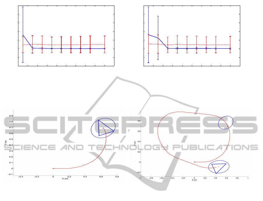
5.1 SLAM Results in Simulation
We performed a series of experiments in simulation
in order to test the suitability of the proposed SLAM
scheme. Please note the importance of assuring the
convergenceof an EKF-based SLAM algorithm when
a new observation model is introduced. Figure 3(a)
presents the simulation environment 1. The true path
followed by the robot is shown with continuous line,
whereas the odometry is represented in dashed line.
A set of views have been placed randomly along the
trajectory and shown with a dot. Please note that the
placement of the views depends of the appearance of
the images and the ratio R selected. In the simulation
we have placed the views randomly with distances
similar to the real case.
The robot starts the SLAM process at the origin
and performs two turns along the trajectory. The
range, i.e. the capability of computing the observation
z
t
= (φ, β)
T
at a given distance is shown with a dash-
dotted line. The observations obtained by the robot
have been simulated using the observation model pre-
sented in Equation 2 with an added gaussian noise
with σ
φ
= σ
β
= 0.1rad. Figure 3(b) presents the sim-
ulation environment 2, which emulates a typical in-
door environment, where the computation of the ob-
servations is restricted by the walls. We performed
a series of experiments when varying the range of
the observed views. The results are presented in Fig-
ure 4(a) and 4(b), where we present the RMS error in
the trajectory when the range of the sensor is varied.
We compare the EKF solution (continuous line) to the
odometry (dashed line) when compared to the laser-
based ground-truth. We generated different odometry
sets randomly and repeated the experiment 50 times.
In Figure 4(a) we present the mean and 2σ intervals.
As can be observed in Figure 4(a) when the range is
0.5m the uncertainty in the pose grows without bound
and the filter is not able to converge. It can be ob-
served that the RMS error decreases when the sensor
range goes beyond 3m. A similar result is presented
in Figure 4(b), which corresponds to the simulation
environment 2. In this case, nice results are obtained
when the range is over 9m, since the walls restrict the
visibility of the views an makes the convergence of
the filter more difficult. Please note that the results
depend strongly on the placement of the views, plac-
ing more viewsallows to compute a more precise map
and trajectory, however it requires a higher computa-
tional cost.
−5 0 5 10 15 20 25
−5
0
5
10
15
20
X (m)
Y (m)
(a)
−5 0 5 10 15 20
0
5
10
15
20
X (m)
Y (m)
(b)
Figure 3: Figure 3(a) represents the simulation environment
1. The location of the different views in the map is repre-
sented by dots. Figure 3(b) presents the simulation environ-
ment 2.
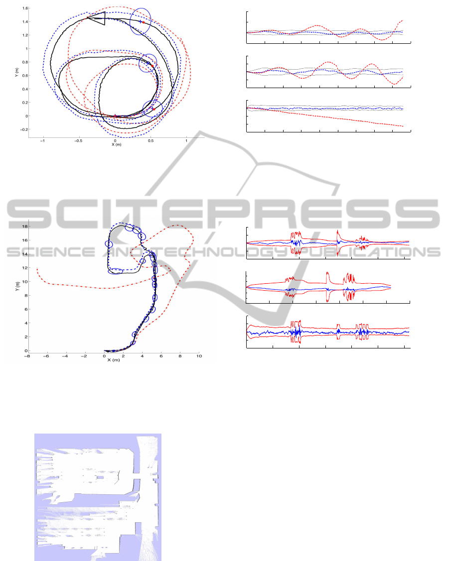
5.2 SLAM with Real Data
In this section we present SLAM results that val-
idate the approach presented here. The robot is
guided through the environment and captures omnidi-
rectional images along the trajectory and laser range
data. Again, in order to compare the results, we use a
laser-based SLAM algorithm, as described in (Stach-
niss et al., 2004). The robot starts by initializing an
omnidirectional image at the origin, as indicated in
Figure 5(a). Next, it starts to move along the trayec-
tory while capturing omnidirectional images. A new
view is initialized a few steps later, as indicated in
Figure 5(a) with an error ellipse. While mapping, the
current image is compared with the rest of the views
in the map, and a set of correspondences is found. In
BUILDING VISUAL MAPS WITH A SINGLE OMNIDIRECTIONAL CAMERA
151
4 6 8 10 12 14 16 18 20 22 24
−20
−10
0
10
20
30
40
50
RMS error in position vs. sensor range
RMS error xy (m)
Sensor range (m)
(a)
4 6 8 10 12 14 16 18 20 22 24
−10
−5
0
5
10
15
20
25
RMS error in position vs. sensor range
RMS error xy (m)
Sensor range (m)
(b)
Figure 4: Figure 4(a) presents the results obtained in the simulation environment 1. Figure 4(b) presents the results obtained
in the simulation environment 2.
(a) (b)
Figure 5: Figure 5(a) and 5(b) present two initial steps in the creation of the map shown in Figure 6.
addition, the similarity ratio (3) is computed. When-
ever the similarity of the current image drops below
δ
R
= 0.5 a new view is created and initialized at the
current robot position. In Figure 5(b) we present the
occurrence of this event, where a third view is initial-
ized. Finally, the robot performs the trajectory shown
in Figure 6(a), where we show with dots the rest of the
poses where the robot decided to initialize a new im-
age. We present with a dashed line the ground truth,
whereas the EKF estimation is drawn with continu-
ous line. The odometry is represented with a dash-
dotted line. It is worth noting that the robot continues
to move inside the same room and is able to compute
observations of the views initialized before. In our
case, the threshold δ
R
was selected experimentally in
order to have a reduced set of views that represent the
environment in a compact manner. If a lower δ
R
is
selected, less images are initialized in the map. On
the contrary, if a greater value of δ
R
is selected (i.e.
0.9), the final map will have a large number of views.
As can be seen in Figure 6(a) once the fourth view is
initialized, no more views are initialized, thus leading
to a compact representation of this environment. In
Figure 6(b) we compare the estimated trajectory with
the ground truth and the odometry at every step of the
trajectory. We present the error in the estimated tra-
jectory (dashed line) with 2σ interval and the error in
the odometry (dash-dotted line).
Figure 7 presents another experiment. In this case,
the robot explores a room, travels through a corri-
dor, goes into a different room and returns. The to-
tal traversed distance is 45m. Figure 7(a) presents
the ground-truth trajectory (dashed line), the odom-
etry (dash-dotted line) and the estimation (continuous
line). The location of the views and its associated un-
certainty is indicated with error ellipses. On Figure
7(b) we present the error in the pose at every step of
the SLAM process with 2σ intervals.
6 CONCLUSIONS
We have presented and approach to the Simultaneous
Localization and Mapping (SLAM) problem using a
single omnidirectional camera. We propose a differ-
ent representation of the environment. Instead of es-
ICINCO 2011 - 8th International Conference on Informatics in Control, Automation and Robotics
152
(a)
0 100 200 300 400 500 600 700 800 900
−1
0
1
2
Error in X (m)
0 100 200 300 400 500 600 700 800 900
−1
−0.5
0
0.5
1
Error in Y (m)
0 100 200 300 400 500 600 700 800 900
−1.5
−1
−0.5
0
0.5
Step
Error in θ (m)
(b)
Figure 6: Figure 6(a) presents the results of SLAM using real data with ground-truth (dashed), estimation (continuous) and
the odometry (dash-dotted). The position of the views is presented with error ellipses. Figure 6(b) presents the error in X, Y
and θ at each time step of the estimation (dashed) and the odometry (dash-dotted).
(a)
0 200 400 600 800 1000 1200
−2
−1
0
1
2
Error in X (m)
0 200 400 600 800 1000 1200 1400
−2
−1
0
1
2
Error in Y (m)
0 200 400 600 800 1000 1200
−0.4
−0.2
0
0.2
0.4
Step number
Error in θ (rad)
(b)
Figure 7: Figure 7(a) presents the results of SLAM using real data with ground-truth (dashed), estimation (continuous) and
the odometry (dash-dotted). The position of the views is presented with error ellipses. Figure 7(b) presents the error in X, Y
and θ at each time step of the estimation (dashed) with a 2σ interval.
Figure 8: The figure presents the occupancy grid map cre-
ated during the experiment shown in Figure 7.
timating the 3D position of a set of visual landmarks
in the environment, we only estimate the position and
orientation of a set of omnidirectional images. Each
omnidirectional image has a set of interest points and
visual descriptors associated to it and describes in a
compact way the environment. Each omnidirectional
image allows the localization of the robot around its
neighbouring. Given two omnidirectional images and
a set of corresponding points, we are able to com-
pute the rotation and translation (up to a scale fac-
tor) between the images. This allows us to propose
an observation model and compute a map and a tra-
jectory. We present localization and SLAM results
using an EKF-based SLAM algorithm, however, we
consider that different SLAM strategies may be used.
We present results obtained in a simulated environ-
ment that validate the SLAM approach. In addition,
we have shown the validity of the approach by using
real data captured with a mobile robot.
BUILDING VISUAL MAPS WITH A SINGLE OMNIDIRECTIONAL CAMERA
153

REFERENCES
Andrew J. Davison, A. J., Gonzalez Cid, Y., and Kita, N.
(2004). Improving data association in vision-based
SLAM. In Proc. of IFAC/EURON, Lisboa, Portugal.
Bay, H., Tuytelaars, T., and Van Gool, L. (2006). SURF:
Speeded up robust features. In Proc. of the ECCV,
Graz, Austria.
Civera, J., Davison, A. J., and Mart´ınez Montiel, J. M.
(2008). Inverse depth parametrization for monocular
slam. IEEE Trans. on Robotics.
Davison, A. J. and Murray, D. W. (2002). Simultaneous lo-
calisation and map-building using active vision. IEEE
Trans. on PAMI.
Fernandez, L., Gil, A., Paya, L., and Reinoso, O. (2010).
An evaluation of weighting methods for appearance-
based monte carlo localization using omnidirectional
images. In Proc. of the ICRA, Anchorage, Alaska.
Gil, A., Martinez-Mozos, O., Ballesta, M., and Reinoso, O.
(2010a). A comparative evaluation of interest point
detectors and local descriptors for visual slam. Ma-
chine Vision and Applications.
Gil, A., Reinoso, O., Ballesta, M., Juli´a, M., and Pay´a, L.
(2010b). Estimation of visual maps with a robot net-
work equipped with vision sensors. Sensors.
Gil, A., Reinoso, O., Martnez-Mozos, O., Stachniss, C., and
Burgard, W. (2006). Improving data association in
vision-based SLAM. In Proc. of the IROS, Beijing,
China.
Grisetti, G., Stachniss, C., Grzonka, S., and Burgard, W.
(2007). A tree parameterization for efficiently com-
puting maximum likelihood maps using gradient de-
scent. In Proc. of RSS, Atlanta, Georgia.
Harris, C. G. and Stephens, M. (1988). A combined corner
and edge detector. In Proc. of Alvey Vision Confer-
ence, Manchester, UK.
Hartley, R. and Zisserman, A. (2004). Multiple View Geom-
etry in Computer Vision. Cambridge University Press.
Jae-Hean, K. and Myung Jin, C. (2003). Slam with omni-
directional stereo vision sensor. In Proc. of the IROS,
Las Vegas (Nevada).
Joly, C. and Rives, P. (2010). Bearing-only SAM using a
minimal inverse depth parametrization. In Proc. of
ICINCO, Funchal, Madeira (Portugal).
Kawanishi, R., Yamashita, A., and Kaneko, T. (2008). Con-
struction of 3D environment model from an omni-
directional image sequence. In Proc. of the Asia Inter-
national Symposium on Mechatronics 2008, Sapporo,
Japan.
Konolige, K., Bowman, J., Chen, J., and Mihelich, P.
(2010). View-based maps. IJRR.
Lowe, D. (2004). Distinctive image features from scale-
invariant keypoints. International Journal of Com-
puter Vision.
Montemerlo, M., Thrun, S., Koller, D., and Wegbreit, B.
(2002). Fastslam: a factored solution to the simulta-
neous localization and mapping problem. In Proc. of
the 18th national conference on Artificial Intelligence,
Edmonton, Canada.
Murillo, A. C., Guerrero, J. J., and Sag¨u´es, C. (2007). SURF
features for efficient robot localization with omnidi-
rectional images. In Proc. of the ICRA, San Diego,
USA.
Neira, J. and Tard´os, J. D. (2001). Data association in
stochastic mapping using the joint compatibility test.
IEEE Trans. on Robotics and Automation.
Nister, D. (2003). An efcient solution to the five-point rela-
tive pose problem. In Proc. of the IEEE CVPR, Madi-
son, USA.
Nist´er, D. (2005). Preemptive RANSAC for live structure
and motion estimation. Machine Vision and Applica-
tions.
Scaramuzza, D., Fraundorfer, F., and Siegwart, R. (2009).
Real-time monocular visual odometry for on-road ve-
hicles with 1-point RANSAC. In Proc. of the ICRA,
Kobe, Japan.
Scaramuzza, D., Martinelli, A., and Siegwart, R. (2006).
A toolbox for easily calibrating omnidirectional cam-
eras. In Proc. of the IROS, Beijing, China.
Se, S., Lowe, D., and Little, J. (2001). Vision-based mobile
robot localization and mapping using scale-invariant
features. In Proc. of the ICRA, Seoul, Korea.
Stachniss, C., Grisetti, G., Haehnel, D., and Burgard, W.
(2004). Improved Rao-Blackwellized mapping by
adaptive sampling and active loop-closure. In Proc.
of the SOAVE, Ilmenau, Germany.
Stewenius, H., Engels, C., and Nister, D. (2006). Recent de-
velopments on direct relative orientation. ISPRS Jour-
nal of Photogrammetry and Remote Sensing.
ICINCO 2011 - 8th International Conference on Informatics in Control, Automation and Robotics
154
