POST-PROCESSING ASSOCIATION RULES WITH CLUSTERING

AND OBJECTIVE MEASURES

Veronica Oliveira de Carvalho

Instituto de Geoci

encias e Ci

encias Exatas, UNESP - Univ Estadual Paulista, Rio Claro, Brazil

Fabiano Fernandes dos Santos, Solange Oliveira Rezende

Instituto de Ci

encias Matem

aticas e de Computac¸

ao, USP - Universidade de S

ao Paulo, S

ao Carlos, Brazil

Keywords:

Association rules, Post-processing, Clustering and objective measures.

Abstract:

The post-processing of association rules is a difﬁcult task, since a large number of patterns can be obtained.

Many approaches have been developed to overcome this problem, as objective measures and clustering, which

are respectively used to: (i) highlight the potentially interesting knowledge in domain; (ii) structure the domain,

organizing the rules in groups that contain, somehow, similar knowledge. However, objective measures don’t

reduce nor organize the collection of rules, making the understanding of the domain difﬁcult. On the other

hand, clustering doesn’t reduce the exploration space nor direct the user to ﬁnd interesting knowledge, making

the search for relevant knowledge not so easy. This work proposes the PAR-COM (Post-processing Asso-

ciation Rules with Clustering and Objective Measures) methodology that, combining clustering and objective

measures, reduces the association rule exploration space directing the user to what is potentially interesting.

Thereby, PAR-COM minimizes the user’s effort during the post-processing process.

1 INTRODUCTION

Association rules are widely used in many distinct do-

main problems (see (Semenova et al., 2001; Fonseca

et al., 2003; Aggelis, 2004; Metwally et al., 2005;

Domingues et al., 2006; Zhang and Gao, 2008; Ra-

jasekar and Weng, 2009; Changguo et al., 2009)) due

to its ability to discover the frequent relationships that

occur among sets of items stored in databases. Al-

though this characteristic along with its inherent com-

prehensibility motivates its use, the main weakness of

association technique occurs when it is necessary to

analyze the mining result. The huge number of ru-

les that are generated makes the user exploration a

difﬁcult task. Many approaches have been developed

to overcome this problem, as Querying (Q), Evalua-

tion Measures (EM), Pruning (P), Summarizing (S)

and Grouping (G) (Baesens et al., 2000; Jorge, 2004;

Natarajan and Shekar, 2005; Zhao et al., 2009). These

post-processing approaches aid the exploration pro-

cess by reducing the exploration space (RES), as Q,

P and S, by directing the user to what is potentially

interesting (DUPI), as EM, or by structuring the do-

main (SD), as G.

One of the more popular approaches to estimate

the interestingness of a rule is the application of eva-

luation measures (Natarajan and Shekar, 2005; Zhao

et al., 2009). These measures are usually classiﬁed as

objective or subjective. The objective measures de-

pend exclusively on the structure pattern and the data

used in the process of knowledge extraction, while the

subjective measures depend fundamentally on the ﬁ-

nal user’s interest and/or needs. Therefore, the objec-

tive measures are more general and independent on

the domain in which the data mining process is car-

ried out. (Geng and Hamilton, 2006; Ohsaki et al.,

2004; Tan et al., 2004) describe many objective mea-

sures besides the classics Support and Conﬁdence. In

this approach, the rules are ranked according to a se-

lected measure and an ordered list of potentially inte-

resting knowledge is shown to the user. Although this

DUPI approach highlights the potentially interesting

knowledge, it doesn’t reduce nor organize the collec-

tion of rules, making the understanding of the domain

difﬁcult.

Grouping is a relevant approach related to SD,

since it organizes the rules in groups that contain,

somehow, similar knowledge. These groups improve

Carvalho V., Santos F. and Rezende S..

POST-PROCESSING ASSOCIATION RULES WITH CLUSTERING AND OBJECTIVE MEASURES.

DOI: 10.5220/0003457500540063

In Proceedings of the 13th International Conference on Enterprise Information Systems (ICEIS-2011), pages 54-63

ISBN: 978-989-8425-53-9

 2011 SCITEPRESS (Science and Technology Publications, Lda.)

the presentation of the mined patterns, providing the

user a view of the domain to be explored (Reynolds

et al., 2006; Sahar, 2002). However, this approach

doesn’t reduce the exploration space nor direct the

user to ﬁnd interesting knowledge, making the search

for ﬁnding relevant knowledge not so easy. Group-

ing can be done: (i) based on a user criteria; (ii) by

using a clustering technique. In case (i) the user des-

cribes how the groups will be formed; for example,

the user can specify that rules that have the same con-

sequent will be grouped together. In case (ii) the user

“let the rules speak for themselves” (Natarajan and

Shekar, 2005).

Clustering is the process of ﬁnding groups in data

(Kaufman and Rousseeuw, 1990). A cluster is a col-

lection of objects that are similar to each other within

the group and dissimilar towards the objects of the

other groups

. Many steps have to be done in a

clustering process as: (i) the selection of a simila-

rity/dissimilarity measure, used to calculate the pro-

ximity among the objects; (ii) the selection/execution

of a clustering algorithm, which are basically divided

in two families: partitional and hierarchical (Kaufman

and Rousseeuw, 1990).

Considering the exposed arguments, this work

proposes the PAR-COM (Post-processing Associa-

tion Rules with Clustering and Objective Measures)

methodology that, by combining clustering (SD) and

objective measures (DUPI), reduces the association

rule exploration space by directing the user to what

is potentially interesting. Thus, PAR-COM improves

the post-processing process since it adheres RES and

DUPI. Besides, different from the approaches related

to RES, PAR-COM doesn’t only show the user a re-

duced space through a small subset of groups but also

highlights the potentially interesting knowledge.

The paper is structured as follows: Section 2 pre-

sents some concepts and related works; Section 3

the PAR-COM methodology; Section 4 the conﬁgu-

rations used in experiments to apply PAR-COM; Sec-

tion 5 the results and discussion; Section 6 the con-

clusions and future works.

2 RELATED WORKS

Since PAR-COM combines clustering and objetive

measures, this section presents some works related to

the clustering approach. The works regarding objec-

tive measures are all associated with the ranking of

rules and due to its simplicity are not here described.

The words cluster and group will be used as synony-

mous in this work.

In order to structure the extracted knowledge, dif-

ferent clustering strategies have been used for post-

processing association rules. (Reynolds et al., 2006)

propose to group partially classiﬁcation rules ob-

tained by two algorithms proposed by them. In this

case, all the rules have the same consequent, i.e.,

the clustering is done taking into accounting the an-

tecedent of the rules. Although the kind of rule con-

sidered in their work is not association, the idea is

the same: the only difference is that all the rules con-

tain the same consequent. Clustering is demonstrated

through partitional (K-means, PAM, CLARANS) and

hierarchical (AGNES) algorithms using Jaccard as the

similarity measure. The Jaccard between two rules r

and s, presented in Equation 1, is calculated conside-

ring the common transactions (t) the rules match (in

our work we refer this similarity measure as Jaccard

with Rules by Transactions (J-RT)). A rule matches a

transaction t if all the rule’s items are contained in t.

J-RT(r,s)=

{t matched by r} ∩ {t matched by s}

{t matched by r} ∪ {t matched by r}

(1)

(Jorge, 2004) demonstrates the use of cluste-

ring through hierarchical algorithms (Single Linkage,

Complete Linkage, Average Linkage) using Jaccard

as the similarity measure. In this case, the Jaccard

between two rules r and s, presented in Equation 2,

is calculated considering the items the rules share (in

our work we refer to this measure as Jaccard with Ru-

les by Items (J-RI)).

J-RI(r,s)=

{items in r}∩ {items in s}

{items in r}∪ {items in r}

(2)

(Toivonen et al., 1995) propose a similarity mea-

sure based on transactions and use a density algorithm

to do the clustering of the rules. In their work it is

considered that all rules contain the same consequent,

i.e., as in (Reynolds et al., 2006) the clustering is done

taking into account the antecedent of the rules. (Sa-

har, 2002) also proposes a similarity measure based

on transactions considering the (Toivonen et al., 1995)

work, although it uses a hierarchical algorithm to do

the clustering. However the algorithm is not men-

tioned and, in this case, it is considered that the rules

contain distinct consequents.

It is important to observe that all the described

works, related to SD, are only concerned with the

domain organization. Thus, a methodology as PAR-

COM that take it as an advantage to reduce the explo-

ration space, by directing the user to relevant know-

ledge, is useful.

POST-PROCESSING ASSOCIATION RULES WITH CLUSTERING AND OBJECTIVE MEASURES

3 PAR-COM METHODOLOGY

The PAR-COM (Post-processing Association Rules

with Clustering and Objective Measures) methodo-

logy aims at combining clustering and objetive mea-

sures to reduce the association rule exploration space

directing the user to what is potentially interesting.

For this purpose, PAR-COM considers that there is

a subset of groups that contains all the h-top interes-

ting rules, so that a small number of groups have to

be explored. The h-top interesting rules are the h ru-

les that have the highest values regarding an objec-

tive measure, where h is a number to be chosen. Be-

sides, it is also considered that if some rules within

a group express interesting knowledge, than the other

rules within the same group also tend to express inte-

resting knowledge. This assumption is taken conside-

ring the concept of cluster: a collection of objects that

are similar to one another. So, if the rules are simi-

lar regarding a similarity measure, an interesting rule

within a group indicates that its similar rules are also

potentially interesting. Based on the exposed argu-

ments, PAR-COM can reduce the exploration space

by directing the user to the groups that are ideally in-

teresting. As as consequence, PAR-COM can allow

the discovery of additional interesting knowledge in-

side these groups.

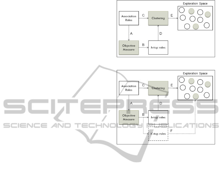
The PAR-COM methodology, presented in Fi-

gure 1, is described as follows:

Step A: the value of an objective measure is com-

puted for all rules in the association set.

Step B: the h-top rules is selected considering the

computed values.

Step C: after selecting a clustering algorithm and a

similarity measure the rule set is clustered.

Step D: a search is done to ﬁnd out the clusters that

contain one or more h-top rules selected in Step B.

These clusters are the ones that contain the poten-

tially interesting knowledge (PIK) of the domain.

The more h-top rules a cluster has the more inte-

resting it is.

Step E: only the m ﬁrst interesting clusters are shown

to the user, who is directed to a reduced explo-

ration space that contains the PIK of the domain,

where m is a number to be chosen.

As will be noted in the results presented in Sec-

tion 5, the combination of clustering with objective

measures used in PAR-COM aids the post-processing

process, minimizing the user’s effort.

Figure 1: The PAR-COM methodology.

Figure 2: Step F: a validation step in the PAR-COM metho-

dology.

4 EXPERIMENTS

Some experiments were carried out to evaluate the

performance of PAR-COM. However, in order to va-

lidate the results shown in Section 5 an additional step

was added to the methodology, as presented in Fi-

gure 2. Step F considers all the h’-top interesting

rules to be also selected in Step B. The h’-top rules

are the ﬁrst h rules that immediately follow the previ-

ously selected h-top rules. Thus, the aim of Step F is

to demonstrate that the m clusters shown to the user

really contain PIK. For this purpose, a search is done

to ﬁnd out if these m clusters contain one or more h’-

top rules. It is expected that these m clusters cover all

the h’-top rules, since by deﬁnition a cluster is a col-

lection of objects that are similar to one another. So,

as mentioned before, if the rules are similar regarding

a similarity measure, an interesting rule inside a group

indicates that its similar rules are also potentially inte-

resting. It is important to note that PAR-COM doesn’t

aid the exploration as an ordered list of PIK, which is

the case when objective measures are used. For that

reason, PAR-COM can allow the discovery of addi-

tional interesting knowledge inside the m groups.

The two data sets used in experiments are pre-

ICEIS 2011 - 13th International Conference on Enterprise Information Systems

Table 1: Details of the data sets used in experiments.

Data set # of transactions # of distinct items Brief description

Adult 48842 115 This set is a R pre-processed version for associa-

tion mining of the “Adult” database available in UCI

(Frank and Asuncion, 2010). It was originally used to

predict whether income exceeds USD 50K/yr based

on census data.

Income 6876 50 This set is also a R pre-processed version for associa-

tion mining of the “Marketing” database available in

(Hastie et al., 2009). It was originally used to predict

the anual income of household from demographics at-

tributes.

sented in Table 1. These data sets are available in

R Project for Statistical Computing

through “arules”

package

. For both data sets the rules were mined

using an Apriori implementation developed by Chris-

tian Borgelt

with a maximum number of 5 items

per rule and excluding the rules of type T RUE ⇒ X ,

where X is an item in the data set. With the Adult

data set 6508 rules were generated using a minimum

support of 10% and a minimum conﬁdence of 50%

and with Income 3714 rules considering a minimum

support of 17% and a minimum conﬁdence of 50%.

These parameter values, as those presented below,

were chosen experimentally.

Since the works described in Section 2 only use

one family of clustering algorithms and one simila-

rity measure to cluster the association rules, it was de-

cided to apply PAR-COM with one algorithm of each

family and with the two most used similarity mea-

sures (J-RI and J-RT (Equations 1 and 2)). The Par-

titioning Around Medoids (PAM) was chosen within

the partitional family and the Average Linkage within

the hierarchical family. In the partitional case, a

medoid algorithm was chosen because the aim is to

cluster the more similar rules in one group; thus, the

ideal is that the centroid group be a rule and not, for

example, the mean, as in the K-means algorithm. In

the hierarchical case, the traditional algorithms were

applied (Single, Complete and Average) and the one

that had the best performance is here presented. PAM

was executed with k ranging between 6 to 15. The

dendrograms generated by Average Linkage were cut

in the same ranges (6 to 15).

To apply PAR-COM it was also necessary to

choose the values of h (Step B), m (Step E) and an

objective measure (Step A). h was set to 15, the high-

est value of k, because we want to evaluate if the 15-

top rules were spread among the groups (one in each

http://www.r-project.org/.

http://cran.r-project.org/web/packages/arules/index.html.

http://www.borgelt.net/apriori.html.

group) or concentrated in little groups (as expected

by the PAR-COM methodology). m was set to 3, half

of the minimum value of k, because we want to eva-

luate the exploration space reduction considering only

50% of the groups. To evaluate the behavior of the

objective measures in the PAR-COM methodology,

6 measures were chosen among the ones described

in (Tan et al., 2004): Certainty Factor (CF), Collec-

tive Strength (CS), Gini Index (GI), Laplace (L), Lift

(also known as Interest Factor) and Novelty (Nov)

(also known as Piatetsky-Shapiro’s, Rule Interest or

Leverage). These measures were chosen because they

are more used than the others in the post-processing

works found in literature (see (Zhao et al., 2009)). Be-

sides, it is expected that any measure produces good

results. Table 2 summarizes the conﬁgurations ap-

plied to evaluate PAR-COM.

Table 2: Conﬁgurations used to evaluate PAR-COM.

Data Adult; Income

sets

Algorithms PAM; Average Linkage

Similarity J-RI; J-RT

measures

k 6 to 15

h 15

m 3

Objective CF; CS; GI; L; Lift; Nov

measures

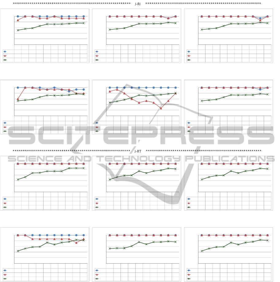
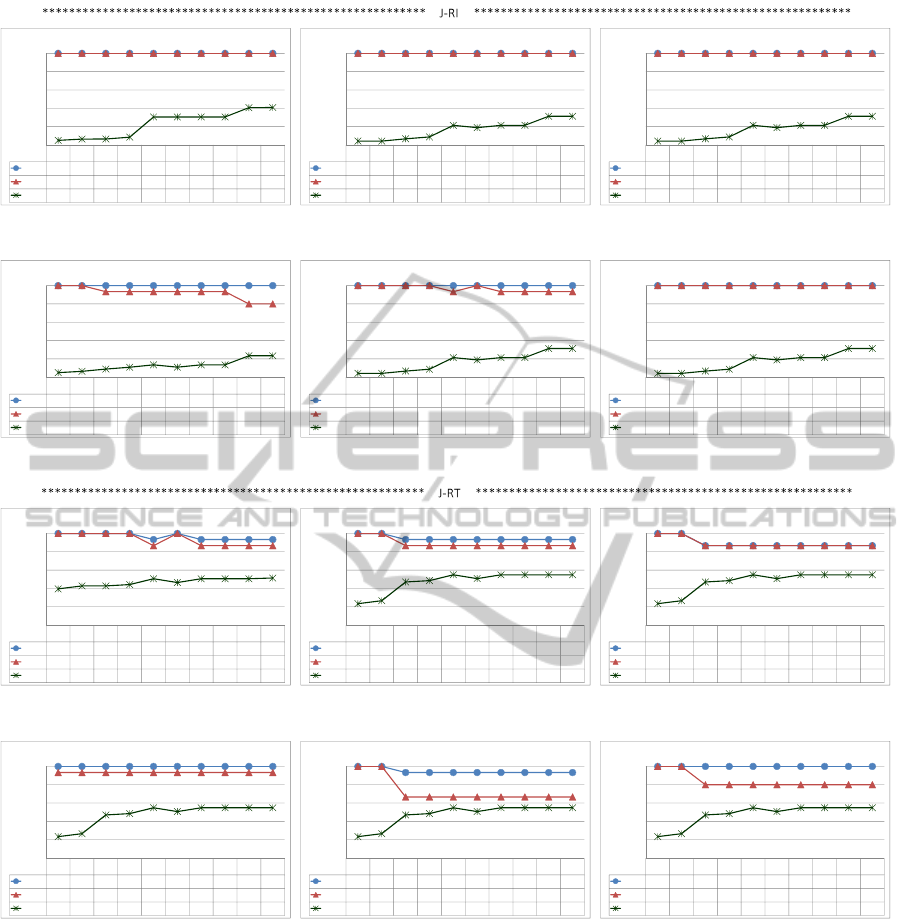
5 RESULTS AND DISCUSSION

Considering the conﬁgurations presented in Table 2,

PAR-COM was applied and the results are presented

in Figures 4, 5, 6 and 7. The results were grouped by

algorithm for each data set. Figures 4 and 6 present

the results for the Adult data set using, respectively,

PAM and Average Linkage and Figures 5 and 7 for

Income also using, respectively, the same algorithms.

Each ﬁgure contains 12 sub-ﬁgures: 6 related to the

POST-PROCESSING ASSOCIATION RULES WITH CLUSTERING AND OBJECTIVE MEASURES

J-RI similarity measure and 6 to J-RT; each group of

these 6 ﬁgures corresponds to an objective measure.

The x axis of each graphic represents the range con-

sidered for k. The y axis represents the percentage of

h-top and h’-top rules contained in the m ﬁrst interes-

ting clusters (lines h-top and h’-top) and also the per-

centage of reduction in the exploration space (line R).

Each graphic title indicates the conﬁguration used.

In order to facilitate the interpretation of the

graphics consider Figure 3 (an enlarged version of

Figure 4(g)). It can be observed that: (i) the ﬁrst

3 interesting clusters (m=3) contain, for each k, all

(100%) the 15-top rules (h=15) using J-RT with CF;

(ii) the ﬁrst 3 interesting clusters contain, for each k,

all (100%) the 15’-top rules (h=15); thus, by the va-

lidation step (Step F), these 3 clusters are ideal the 3

most interesting subsets; (iii) for k=15, for example,

the ﬁrst 3 interesting clusters cover 16% (100%-84%)

of the rules, leading to a reduction of 84% in the ex-

ploration space; in order words, if the user explores

these 3 clusters, he will explore 16% of the rule’s

space.

6 7 8 9 10 11 12 13 14 15

top

100%

h'-top

100% 100% 100% 100% 100% 100% 100% 100% 100% 100%

44% 52% 67% 68% 73% 73% 73% 84% 84% 84%

20%

40%

60%

80%

100%

ADULT :: PAM :: J-RT :: CF

Figure 3: PAM result in the Adult data set using J-RT and

CF.

Evaluating the results, in relation to PAM algo-

rithm, it can be noticed that:

• in Figure 4 the J-RT similarity measure presen-

ted better results compared with J-RI in rela-

tion to the h-top and h’-top rules (compare 4(a)

with 4(g), 4(b) with 4(h), 4(c) with 4(i), 4(d)

with 4(j), 4(e) with 4(k) and 4(f) with 4(l)). How-

ever, J-RI and J-RT had a similar behavior regar-

ding the exploration space reduction. In J-RT all

the objective measures presented similar results

regarding h and h’ different from J-RI that had the

worst performance in Laplace and Lift. Besides,

in both cases, high values of k give high reduc-

tions and a good performance related to the h and

h’-top rules.

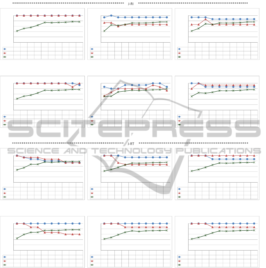
• in Figure 5 the J-RT similarity measure presented,

in almost all the cases, better results compared

with J-RI in relation to the h-top and h’-top ru-

les (compare 5(a) with 5(g), 5(b) with 5(h), 5(c)

with 5(i), 5(d) with 5(j), 5(e) with 5(k) and 5(f)

with 5(l)). However, J-RI and J-RT had a similar

behavior regarding the exploration space reduc-

tion. Certainty Factor and Laplace generated bet-

ter results than the others in J-RI regarding h and

h’; in J-RT, Gini Index, Lift and Novelty generated

better results than the others regarding h and h’.

Besides, in both cases, high values of k give high

reductions and a good performance related to the

h and h’-top rules.

Summarizing the results in Figures 4 and 5, it can

be seen that with the PAM algorithm the similarity

measure that had the best performance was J-RT re-

garding h and h’. However, considering the explo-

ration space reduction, both similarity measures pre-

sented similar behavior. On the other hand, in relation

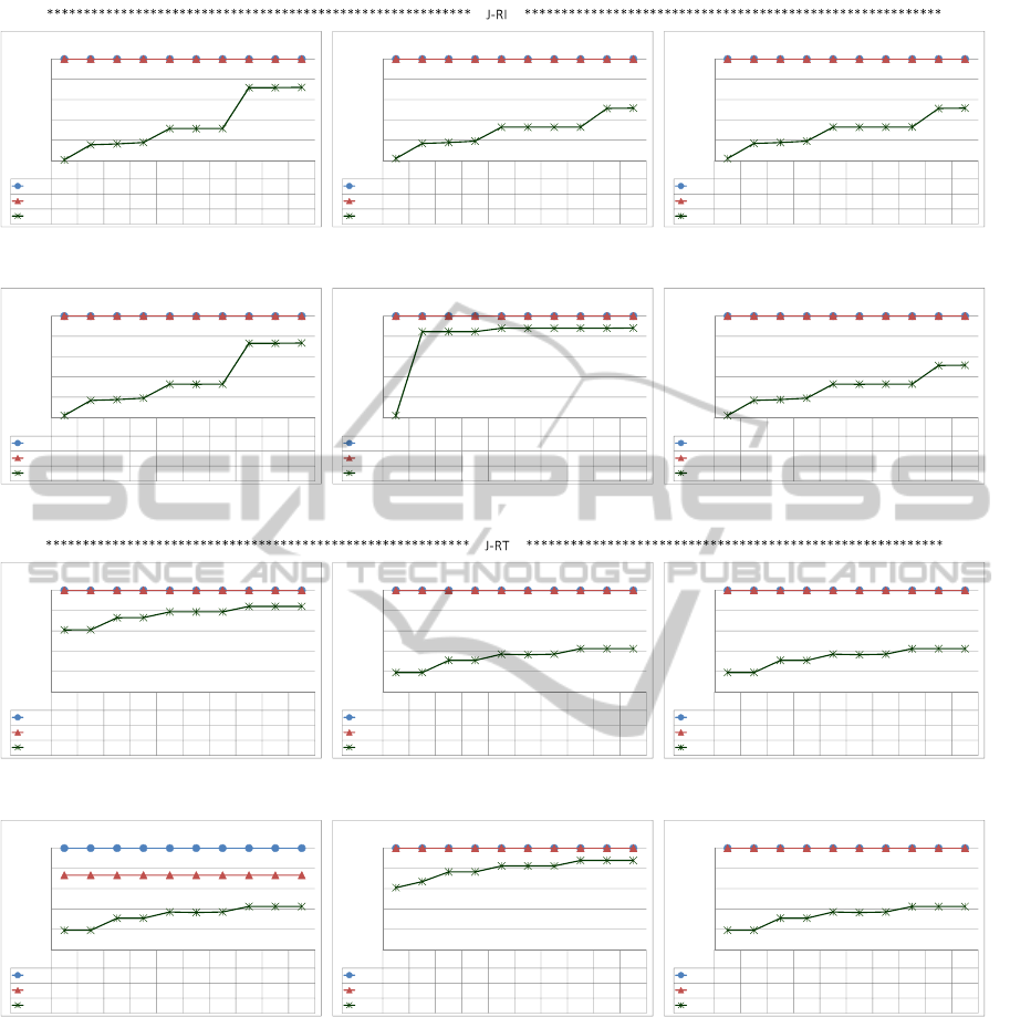
to Average algorithm, it can be noticed that:

• in Figure 6 both J-RI and J-RT presented good re-

sults in relation to the h-top and h’-top rules in

all the used objective measures. In almost all the

cases, J-RI had a little better performance than

J-RT considering the exploration space reduction

for high values of k (compare 6(a) with 6(g), 6(b)

with 6(h), 6(c) with 6(i), 6(d) with 6(j), 6(e)

with 6(k) and 6(f) with 6(l)). Besides, in both

cases, high values of k give high reductions and

a good performance related to the h and h’-top ru-

les.

• in Figure 7 both J-RI and J-RT presented good

results in relation to the h-top and h’-top rules

in almost all the used objective measures (excep-

tions were Figures 7(k) and 7(l)), although J-RI

had a better performance than J-RT (compare 7(a)

with 7(g), 7(b) with 7(h), 7(c) with 7(i), 7(d)

with 7(j), 7(e) with 7(k) and 7(f) with 7(l)). In

all the cases J-RT had a better performance than

J-RI considering the exploration space reduction.

Besides, in both cases, high values of k give high

reductions and a good performance related to the

h and h’-top rules.

Summarizing the results in Figures 6 and 7, it can

be seen that with the Average algorithm the simila-

rity measure that had the best performance was J-RI

regarding h and h’, although J-RT had presented si-

milar behavior in many cases. However, considering

the exploration space reduction, none of the simila-

rity measures won in both data sets. Thus, since PAM

had a better performance with J-RT and Average with

J-RI, comparing the results of PAM using J-RT (Fi-

gures 4(g) to 4(l) and 5(g) to 5(l)) with Average using

ICEIS 2011 - 13th International Conference on Enterprise Information Systems

6 7 8 9 10 11 12 13 14 15

top

100%

h'-top

87% 100% 100% 93% 93% 100% 93% 93% 93% 93%

51% 55% 58% 66% 72% 72% 72% 74% 76% 76%

20%

40%

60%

80%

100%

ADULT :: PAM :: J-RI :: CF

(a)

6 7 8 9 10 11 12 13 14 15

top

100%

93%

100%

h'-top

100% 100% 100% 100% 100% 100% 100% 100% 93% 100%

53% 55% 58% 66% 74% 73% 74% 74% 78% 76%

20%

40%

60%

80%

100%

ADULT :: PAM :: J-RI :: CS

(b)

6 7 8 9 10 11 12 13 14 15

top

100%

93%

100%

h'-top

100% 100% 100% 100% 100% 100% 100% 100% 87% 100%

53% 55% 58% 66% 74% 73% 74% 74% 78% 76%

20%

40%

60%

80%

100%

ADULT :: PAM :: J-RI :: GI

(c)

6 7 8 9 10 11 12 13 14 15

top

100%

93%

100%

93%

87%

93%

h'-top

60% 100% 100% 93% 93% 93% 93% 93% 80% 80%

53% 55% 58% 66% 72% 72% 72% 74% 78% 76%

20%

40%

60%

80%

100%

ADULT :: PAM :: J-RI :: L

(d)

6 7 8 9 10 11 12 13 14 15

top

100%

h'-top

87% 93% 80% 60% 47% 53% 47% 27% 53% 80%

47% 51% 57% 64% 73% 71% 73% 75% 78% 80%

20%

40%

60%

80%

100%

ADULT :: PAM :: J-RI :: LIFT

(e)

6 7 8 9 10 11 12 13 14 15

top

100%

93%

100%

h'-top

100% 100% 100% 100% 100% 100% 100% 100% 100% 100%

53% 55% 58% 66% 74% 73% 74% 74% 78% 76%

20%

40%

60%

80%

100%

ADULT :: PAM :: J-RI :: NOV

(f)

6 7 8 9 10 11 12 13 14 15

top

100%

h'-top

100% 100% 100% 100% 100% 100% 100% 100% 100% 100%

44% 52% 67% 68% 73% 73% 73% 84% 84% 84%

20%

40%

60%

80%

100%

ADULT :: PAM :: J-RT :: CF

(g)

6 7 8 9 10 11 12 13 14 15

top

100%

h'-top

100% 100% 100% 100% 100% 100% 100% 100% 100% 100%

44% 52% 58% 59% 74% 67% 74% 77% 83% 82%

20%

40%

60%

80%

100%

ADULT :: PAM :: J-RT :: CS

(h)

6 7 8 9 10 11 12 13 14 15

top

100%

h'-top

100% 100% 100% 100% 100% 100% 100% 100% 100% 100%

44% 52% 58% 59% 74% 67% 74% 77% 83% 82%

20%

40%

60%

80%

100%

ADULT :: PAM :: J-RT :: GI

(i)

6 7 8 9 10 11 12 13 14 15

top

100%

h'-top

100% 100% 87% 87% 87% 87% 87% 87% 73% 87%

44% 52% 58% 59% 74% 67% 74% 77% 83% 82%

20%

40%

60%

80%

100%

ADULT :: PAM :: J-RT :: L

(j)

6 7 8 9 10 11 12 13 14 15

top

100%

h'-top

100% 100% 100% 100% 100% 100% 100% 100% 100% 100%

53% 54% 54% 61% 76% 68% 76% 76% 78% 76%

20%

40%

60%

80%

100%

ADULT :: PAM :: J-RT :: LIFT

(k)

6 7 8 9 10 11 12 13 14 15

top

100%

h'-top

100% 100% 100% 100% 100% 100% 100% 100% 100% 100%

44% 52% 58% 59% 74% 67% 74% 77% 83% 82%

20%

40%

60%

80%

100%

ADULT :: PAM :: J-RT :: NOV

(l)

Figure 4: PAM’s results in the ADULT data set.

J-RI (Figures 6(a) to 6(f) and 7(a) to 7(f)), it can be

noticed that:

• in the Adult data set both algorithms had good re-

sults and similar behavior regarding h and h’: in

all the cases, 100% of recovery in the 3 interes-

ting clusters (m=3) regarding h; in almost all the

cases, 100% of recovery in the 3 interesting clus-

ters (m=3) regarding h’ (exception to Figure 4(j)).

However, PAM had better results considering the

reduction exploration space (above 80% for high

values of k).

• in the Income data set the Average algorithm had

good results and a better performance compared

with PAM regarding h and h’: in all the cases,

100% of recovery in the 3 interesting clusters

(m=3) regarding h; in almost all the cases, 100%

of recovery in the 3 interesting clusters (m=3) re-

garding h’ (exception to Figures 7(d) and 7(e)).

However, PAM had better results considering the

reduction exploration space (above 70% for high

POST-PROCESSING ASSOCIATION RULES WITH CLUSTERING AND OBJECTIVE MEASURES

6 7 8 9 10 11 12 13 14 15

top

100%

h'-top

100% 100% 100% 100% 100% 100% 100% 100% 100% 100%

42% 52% 56% 64% 74% 73% 74% 75% 77% 76%

20%

40%

60%

80%

100%

INCOME :: PAM :: J-RI :: CF

(a)

6 7 8 9 10 11 12 13 14 15

top

93%

100%

93%

h'-top

73% 73% 60% 67% 67% 67% 67% 67% 67% 67%

42% 65% 63% 66% 72% 72% 72% 73% 76% 76%

20%

40%

60%

80%

100%

INCOME :: PAM :: J-RI :: CS

(b)

6 7 8 9 10 11 12 13 14 15

top

93%

87%

h'-top

67% 67% 87% 67% 67% 67% 67% 67% 67% 67%

42% 52% 69% 66% 72% 72% 72% 73% 76% 76%

20%

40%

60%

80%

100%

INCOME :: PAM :: J-RI :: GI

(c)

6 7 8 9 10 11 12 13 14 15

top

100%

93%

h'-top

100% 100% 100% 100% 100% 100% 100% 100% 87% 100%

42% 52% 56% 64% 74% 73% 74% 75% 77% 76%

20%

40%

60%

80%

100%

INCOME :: PAM :: J-RI :: L

(d)

6 7 8 9 10 11 12 13 14 15

top

87%

80%

93%

100%

87%

h'-top

53% 67% 80% 80% 80% 80% 80% 93% 87% 73%

51% 52% 68% 71% 74% 73% 74% 76% 76% 79%

20%

40%

60%

80%

100%

INCOME :: PAM :: J-RI :: LIFT

(e)

6 7 8 9 10 11 12 13 14 15

top

100%

87%

h'-top

80% 100% 93% 93% 93% 93% 93% 93% 93% 93%

51% 65% 63% 66% 72% 72% 72% 73% 76% 76%

20%

40%

60%

80%

100%

INCOME :: PAM :: J-RI :: NOV

(f)

6 7 8 9 10 11 12 13 14 15

top

100%

93%

87%

80%

73%

h'-top

100% 93% 93% 93% 87% 87% 87% 73% 73% 73%

46% 54% 67% 67% 76% 75% 76% 77% 78% 78%

20%

40%

60%

80%

100%

INCOME :: PAM :: J-RT :: CF

(g)

6 7 8 9 10 11 12 13 14 15

top

100%

93%

h'-top

100% 100% 73% 67% 67% 67% 67% 67% 67% 67%

42% 48% 56% 65% 72% 71% 72% 74% 74% 74%

20%

40%

60%

80%

100%

INCOME :: PAM :: J-RT :: CS

(h)

6 7 8 9 10 11 12 13 14 15

top

100%

87%

h'-top

100% 100% 100% 100% 100% 100% 100% 100% 100% 100%

42% 48% 56% 65% 72% 71% 72% 74% 74% 74%

20%

40%

60%

80%

100%

INCOME :: PAM :: J-RT :: GI

(i)

6 7 8 9 10 11 12 13 14 15

top

100%

h'-top

100% 100% 87% 87% 67% 67% 67% 60% 60% 60%

44% 59% 67% 67% 74% 74% 74% 76% 77% 77%

20%

40%

60%

80%

100%

INCOME :: PAM :: J-RT :: L

(j)

6 7 8 9 10 11 12 13 14 15

top

100%

h'-top

100% 100% 100% 87% 87% 87% 87% 87% 87% 87%

42% 48% 58% 67% 73% 70% 73% 73% 73% 74%

20%

40%

60%

80%

100%

INCOME :: PAM :: J-RT :: LIFT

(k)

6 7 8 9 10 11 12 13 14 15

top

100%

h'-top

100% 100% 100% 87% 87% 87% 87% 87% 87% 87%

42% 48% 56% 65% 72% 71% 72% 74% 74% 74%

20%

40%

60%

80%

100%

INCOME :: PAM :: J-RT :: NOV

(l)

Figure 5: PAM’s results in the INCOME data set.

values of k).

Based on the exposed discussion, it can be seen

that the user can apply PAR-COM considering the

combination PAM:J-RT or Average:J-RI. However,

it is important to note that these similarity measures

have a semantic that needs to be explored. That way,

an evaluation with ﬁnal users has to be done to ﬁnd

out which of them better recover the more adequate

subset of groups related to the PIK.

Still discussing the results, it can be observed that

the used objective measures had, broadly, a good per-

formance regarding the h and h’-top rules. The ex-

ceptions, considering percentages below 70, were Fi-

gures 4(d), 4(e), 5(b), 5(c), 5(e), 5(h), 5(j) and 7(k),

which represents approximately only 17% of the

cases. Besides, high values of k give high reductions

and a good performance related to the h and h’-top ru-

les. Thus, we can reduce the exploration space when

using high values of k also maintaining an interesting

subset of rules.

ICEIS 2011 - 13th International Conference on Enterprise Information Systems

6 7 8 9 10 11 12 13 14 15

top

100%

h'-top

100% 100% 100% 100% 100% 100% 100% 100% 100% 100%

1% 15% 16% 18% 31% 31% 31% 72% 72% 72%

20%

40%

60%

80%

100%

ADULT :: AVERAGE :: J-RI :: CF

(a)

6 7 8 9 10 11 12 13 14 15

top

100%

h'-top

100% 100% 100% 100% 100% 100% 100% 100% 100% 100%

2% 17% 18% 19% 33% 33% 33% 33% 51% 52%

20%

40%

60%

80%

100%

ADULT :: AVERAGE :: J-RI :: CS

(b)

6 7 8 9 10 11 12 13 14 15

top

100%

h'-top

100% 100% 100% 100% 100% 100% 100% 100% 100% 100%

2% 17% 18% 19% 33% 33% 33% 33% 51% 52%

20%

40%

60%

80%

100%

ADULT :: AVERAGE :: J-RI :: GI

(c)

6 7 8 9 10 11 12 13 14 15

top

100%

h'-top

100% 100% 100% 100% 100% 100% 100% 100% 100% 100%

2% 17% 18% 19% 33% 33% 33% 73% 73% 73%

20%

40%

60%

80%

100%

ADULT :: AVERAGE :: J-RI :: L

(d)

6 7 8 9 10 11 12 13 14 15

top

100%

h'-top

100% 100% 100% 100% 100% 100% 100% 100% 100% 100%

2% 85% 85% 85% 88% 88% 88% 88% 88% 88%

20%

40%

60%

80%

100%

ADULT :: AVERAGE :: J-RI :: LIFT

(e)

6 7 8 9 10 11 12 13 14 15

top

100%

h'-top

100% 100% 100% 100% 100% 100% 100% 100% 100% 100%

2% 17% 18% 19% 33% 33% 33% 33% 51% 52%

20%

40%

60%

80%

100%

ADULT :: AVERAGE :: J-RI :: NOV

(f)

6 7 8 9 10 11 12 13 14 15

top

100%

h'-top

100% 100% 100% 100% 100% 100% 100% 100% 100% 100%

61% 61% 73% 73% 79% 79% 79% 84% 84% 84%

20%

40%

60%

80%

100%

ADULT :: AVERAGE :: J-RT :: CF

(g)

6 7 8 9 10 11 12 13 14 15

top

100%

h'-top

100% 100% 100% 100% 100% 100% 100% 100% 100% 100%

19% 19% 31% 31% 37% 36% 37% 42% 42% 42%

20%

40%

60%

80%

100%

ADULT :: AVERAGE :: J-RT :: CS

(h)

6 7 8 9 10 11 12 13 14 15

top

100%

h'-top

100% 100% 100% 100% 100% 100% 100% 100% 100% 100%

19% 19% 31% 31% 37% 36% 37% 42% 42% 42%

20%

40%

60%

80%

100%

ADULT :: AVERAGE :: J-RT :: GI

(i)

6 7 8 9 10 11 12 13 14 15

top

100%

h'-top

73% 73% 73% 73% 73% 73% 73% 73% 73% 73%

19% 19% 31% 31% 37% 36% 37% 42% 42% 42%

20%

40%

60%

80%

100%

ADULT :: AVERAGE :: J-RT :: L

(j)

6 7 8 9 10 11 12 13 14 15

top

100%

h'-top

100% 100% 100% 100% 100% 100% 100% 100% 100% 100%

61% 67% 77% 77% 82% 82% 82% 88% 88% 88%

20%

40%

60%

80%

100%

ADULT :: AVERAGE :: J-RT :: LIFT

(k)

6 7 8 9 10 11 12 13 14 15

top

100%

h'-top

100% 100% 100% 100% 100% 100% 100% 100% 100% 100%

19% 19% 31% 31% 37% 36% 37% 42% 42% 42%

20%

40%

60%

80%

100%

ADULT :: AVERAGE :: J-RT :: NOV

(l)

Figure 6: AVERAGE’s results in the ADULT data set.

6 CONCLUSIONS

This work presented the PAR-COM methodology that

by combining clustering (SD) and objective measures

(DUPI) provides a powerful tool to aid the post-

processing process, minimizing the user’s effort du-

ring the exploration process. PAR-COM can present

to the user only a small subset of the rules, provi-

ding a view to what is really interesting. Thereby,

PAR-COM adheres RES and DUPI. PAR-COM has

a good performance, as observed in Section 5, in:

(i) highlighting the potentially interesting knowledge

(PIK), demonstrated through the h’-top rules; (ii) re-

ducing the exploration space. Thus, PAR-COM can

reduce the exploration space without losing PIK, be-

ing a good methodology for post-processing associa-

tion rules.

As a future work, some labeling methodologies

will be studied and implemented that, along with

PAR-COM, will direct the user to the potentially inte-

POST-PROCESSING ASSOCIATION RULES WITH CLUSTERING AND OBJECTIVE MEASURES

6 7 8 9 10 11 12 13 14 15

top

100%

h'-top

100% 100% 100% 100% 100% 100% 100% 100% 100% 100%

5% 6% 6% 8% 31% 31% 31% 31% 41% 41%

20%

40%

60%

80%

100%

INCOME :: AVERAGE :: J-RI :: CF

(a)

6 7 8 9 10 11 12 13 14 15

top

100%

h'-top

100% 100% 100% 100% 100% 100% 100% 100% 100% 100%

4% 4% 7% 9% 21% 19% 21% 21% 31% 31%

20%

40%

60%

80%

100%

INCOME :: AVERAGE :: J-RI :: CS

(b)

6 7 8 9 10 11 12 13 14 15

top

100%

h'-top

100% 100% 100% 100% 100% 100% 100% 100% 100% 100%

4% 4% 7% 9% 21% 19% 21% 21% 31% 31%

20%

40%

60%

80%

100%

INCOME :: AVERAGE :: J-RI :: GI

(c)

6 7 8 9 10 11 12 13 14 15

top

100%

h'-top

100% 100% 93% 93% 93% 93% 93% 93% 80% 80%

5% 6% 9% 11% 13% 11% 13% 13% 23% 23%

20%

40%

60%

80%

100%

INCOME :: AVERAGE :: J-RI :: L

(d)

6 7 8 9 10 11 12 13 14 15

top

100%

h'-top

100% 100% 100% 100% 93% 100% 93% 93% 93% 93%

4% 4% 7% 9% 21% 19% 21% 21% 31% 31%

20%

40%

60%

80%

100%

INCOME :: AVERAGE :: J-RI :: LIFT

(e)

6 7 8 9 10 11 12 13 14 15

top

100%

h'-top

100% 100% 100% 100% 100% 100% 100% 100% 100% 100%

4% 4% 7% 9% 21% 19% 21% 21% 31% 31%

20%

40%

60%

80%

100%

INCOME :: AVERAGE :: J-RI :: NOV

(f)

6 7 8 9 10 11 12 13 14 15

top

100%

93%

100%

93%

h'-top

100% 100% 100% 100% 87% 100% 87% 87% 87% 87%

39% 43% 43% 44% 51% 46% 51% 51% 51% 51%

20%

40%

60%

80%

100%

INCOME :: AVERAGE :: J-RT :: CF

(g)

6 7 8 9 10 11 12 13 14 15

top

100%

93%

h'-top

100% 100% 87% 87% 87% 87% 87% 87% 87% 87%

23% 27% 47% 49% 55% 51% 55% 55% 55% 55%

20%

40%

60%

80%

100%

INCOME :: AVERAGE :: J-RT :: CS

(h)

6 7 8 9 10 11 12 13 14 15

top

100%

87%

h'-top

100% 100% 87% 87% 87% 87% 87% 87% 87% 87%

23% 27% 47% 49% 55% 51% 55% 55% 55% 55%

20%

40%

60%

80%

100%

INCOME :: AVERAGE :: J-RT :: GI

(i)

6 7 8 9 10 11 12 13 14 15

top

100%

h'-top

93% 93% 93% 93% 93% 93% 93% 93% 93% 93%

23% 27% 47% 49% 55% 51% 55% 55% 55% 55%

20%

40%

60%

80%

100%

INCOME :: AVERAGE :: J-RT :: L

(j)

6 7 8 9 10 11 12 13 14 15

top

100%

93%

h'-top

100% 100% 67% 67% 67% 67% 67% 67% 67% 67%

23% 27% 47% 49% 55% 51% 55% 55% 55% 55%

20%

40%

60%

80%

100%

INCOME :: AVERAGE :: J-RT :: LIFT

(k)

6 7 8 9 10 11 12 13 14 15

top

100%

h'-top

100% 100% 80% 80% 80% 80% 80% 80% 80% 80%

23% 27% 47% 49% 55% 51% 55% 55% 55% 55%

20%

40%

60%

80%

100%

INCOME :: AVERAGE :: J-RT :: NOV

(l)

Figure 7: AVERAGE’s results in the INCOME data set.

resting “topics” (PIT) in the domain.

ACKNOWLEDGEMENTS

We wish to thank Fundac¸

ao de Amparo

a Pesquisa

do Estado de S

ao Paulo (FAPESP) for the ﬁnancial

support (process number 2010/07879-0).

REFERENCES

Aggelis, V. (2004). Association rules model of e-banking

services. Data Mining V – Information and Commu-

nication Technologies, 5:46–55.

Baesens, B., Viaene, S., and Vanthienen, J. (2000). Post-

processing of association rules. In KDD’00: Pro-

ceedings of the Special Workshop on Post-processing,

The 6th ACM SIGKDD International Conference on

Knowledge Discovery and Data Mining, pages 2–8.

ICEIS 2011 - 13th International Conference on Enterprise Information Systems

Changguo, Y., Nianzhong, W., Tailei, W., Qin, Z., and

Xiaorong, Z. (2009). The research on the appli-

cation of association rules mining algorithm in net-

work intrusion detection. In Hu, Z. and Liu, Q., edi-

tors, ETCS’09: Proceedings of the 1st International

Workshop on Education Technology and Computer

Science, volume 2, pages 849–852.

Domingues, M. A., Jorge, A. M., and Soares, C. (2006).

Using association rules for monitoring meta-data

quality in web portals. In WAAMD’06: Proceedings

of the II Workshop em Algoritmos e Aplicac¸

oes de Mi-

nerac¸

ao de Dados – SBBD/SBES, pages 105–108.

Fonseca, B. M., Golgher, P. B., Moura, E. S., and Ziviani, N.

(2003). Using association rules to discover search en-

gines related queries. In LA-WEB’03: Proceedings of

the 1st Conference on Latin American Web Congress,

pages 66–71. IEEE Computer Society.

Frank, A. and Asuncion, A. (2010). UCI machine

learning repository. University of California, Irvine,

School of Information and Computer Sciences.

http://archive.ics.uci.edu/ml.

Geng, L. and Hamilton, H. J. (2006). Interestingness mea-

sures for data mining: A survey. In ACM Computing

Surveys, volume 38. ACM Press.

Hastie, T., Tibshirani, R., and Friedman, J. (2009).

The Elements of Statistical Learning: Data Mi-

ning, Inference, and Prediction. Springer Series

in Statistics. Springer, second edition. http://www-

stat.stanford.edu/ tibs/ElemStatLearn/.

Jorge, A. (2004). Hierarchical clustering for thematic

browsing and summarization of large sets of associa-

tion rules. In Berry, M. W., Dayal, U., Kamath, C.,

and Skillicorn, D., editors, SIAM’04: Proceedings of

the 4th SIAM International Conference on Data Mi-

ning. 10p.

Kaufman, L. and Rousseeuw, P. J. (1990). Finding Groups

in Data: An Introduction to Cluster Analysis. Wiley-

Interscience.

Metwally, A., Agrawal, D., and Abbadi, A. E. (2005). Using

association rules for fraud detection in web adverti-

sing networks. In VLDB’05: Proceedings of the 31st

International Conference on Very Large Data Bases,

pages 169–180.

Natarajan, R. and Shekar, B. (2005). Interestingness of

association rules in data mining: Issues relevant to e-

commerce. S

ADHAN

A – Academy Proceedings in En-

gineering Sciences (The Indian Academy of Sciences),

30(Parts 2&3):291–310.

Ohsaki, M., Kitaguchi, S., Okamoto, K., Yokoi, H., and Ya-

maguchi, T. (2004). Evaluation of rule interestingness

measures with a clinical dataset on hepatitis. In Bouli-

caut, J.-F., Esposito, F., Giannotti, F., and Pedreschi,

D., editors, PKDD’04: Proceedings of the 8th Euro-

pean Conference on Principles and Practice of Know-

ledge Discovery in Databases, volume 3202, pages

362–373. Springer-Verlag New York, Inc.

Rajasekar, U. and Weng, Q. (2009). Application of asso-

ciation rule mining for exploring the relationship be-

tween urban land surface temperature and biophysi-

cal/social parameters. Photogrammetric Engineering

& Remote Sensing, 75(3):385–396.

Reynolds, A. P., Richards, G., de la Iglesia, B., and

Rayward-Smith, V. J. (2006). Clustering rules: A

comparison of partitioning and hierarchical clustering

algorithms. Journal of Mathematical Modelling and

Algorithms, 5(4):475–504.

Sahar, S. (2002). Exploring interestingness through clus-

tering: A framework. In ICDM’02: Proceedings of

the IEEE International Conference on Data Mining,

pages 677–680.

Semenova, T., Hegland, M., Graco, W., and Williams,

G. (2001). Effectiveness of mining association ru-

les for identifying trends in large health databases.

In Kurfess, F. J. and Hilario, M., editors, ICDM’01:

Workshop on Integrating Data Mining and Knowledge

Management, The IEEE International Conference on

Data Mining. 12p.

Tan, P.-N., Kumar, V., and Srivastava, J. (2004). Selecting

the right objective measure for association analysis.

Information Systems, 29(4):293–313.

Toivonen, H., Klemettinen, M., Ronkainen, P., H

onen,

K., and Mannila, H. (1995). Pruning and grouping

discovered association rules. Workshop Notes of the

ECML’95 Workshop on Statistics, Machine Learning,

and Knowledge Discovery in Databases, 47–52, ML-

net.

Zhang, J. and Gao, W. (2008). Application of association

rules mining in the system of university teaching ap-

praisal. In ETTANDGRS’08: Proceedings of the In-

ternational Workshop on Education Technology and

Training & International Workshop on Geoscience

and Remote Sensing, volume 2, pages 26–28. IEEE

Computer Society.

Zhao, Y., Zhang, C., and Cao, L. (2009). Post-Mining of

Association Rules: Techniques for Effective Know-

ledge Extraction. Information Science Reference.

372p.

POST-PROCESSING ASSOCIATION RULES WITH CLUSTERING AND OBJECTIVE MEASURES