MODELING, SIMULATION AND CONTROL OF A WATER
RECOVERY AND IRRIGATION SYSTEM
Mohamed Abdelati
Electrical Engineering Department, IUG, Gaza, Palestine
Felix Felgner, Georg Frey
Chair of Automation, Saarland University, Saarbrücken, Germany
Keywords: System modeling, Water recovery, Automation, Modelica.
Abstract: For the modeling and simulation of large water recovery and irrigation systems, standard component models
as found in simulation tool libraries are too complex. In this work, simple models are derived and applied
for the modeling and simulation of a real system. In this system, water for irrigation will be collected by
recovery wells around the wastewater treatment plant infiltration basins located in northern Gaza. There will
be 27 recovery wells to collect the water in a reservoir before being distributed for irrigation via 10 booster
pumps. During summer time, the system is expected to recover and distribute about 50885 m
3
daily. The
model derived in this paper using Modelica helps better understanding the system dynamics and provides a
tool for evaluating the performance of possible control schemes.
1 INTRODUCTION
Daily amounts of about 15000 m
3
of partially treated
wastewater are infiltrated through allocated basins in
northern Gaza. Once the construction of a new
treatment plant is completed, the infiltrated water
will reach an average of 35000 m
3
per day. This
infiltrated water is not suitable for domestic use and
eventually will contaminate the aquifer of all over
northern Gaza (Werner, 2006). However, this water
is suitable for irrigation and is recommended to be
utilized due to the scarce water recourses of Gaza.
Consequently, the Palestinian Water Authority
(PWA) with technical assistance from specialists
proposed the construction of 27 recovery wells
around the infiltration basins. Pumps of 56 kW will
be used in these wells and recovered water will be
collected in a 8000 m
3
reservoir before being
distributed for irrigation via 10 booster pumps, each
with a rating of 350 kW (Ziara, 2010). Recovery
pumps have an expected head of 90 m and a pumping
capacity of 170 m
3
/hr at that head, while booster
pumps have an expected head of 115 m and a
pumping capacity of 750 m
3
/hr at that operating
point. Figure 1 illustrates the layout of the waste
water treatment plant in northern Gaza.
Figure 1: The recovery wells and collection pipes.
The presented work is part of a project which
aims to design a control system for the infiltrated
wastewater recovery. To this end, first a simulation
model is designed based on the physical properties of
the process. This model, using the component-
pipe
reservoir
recovery
well
infiltration
basins
Scale 1:22000
323
Abdelati M., Felgner F. and Frey G..
MODELING, SIMULATION AND CONTROL OF A WATER RECOVERY AND IRRIGATION SYSTEM.
DOI: 10.5220/0003457303230329
In Proceedings of the 8th International Conference on Informatics in Control, Automation and Robotics (ICINCO-2011), pages 323-329
ISBN: 978-989-8425-74-4
Copyright
c
 2011 SCITEPRESS (Science and Technology Publications, Lda.)

oriented modeling language Modelica (Tiller, 2004),
is then used to design and validate proposed
automation strategies.
The paper is organized as follows: Section 2
describes the recovery process and the irrigation
scheme. In Section 3, the modeling is described and
in Section 4, some simulation results of the proposed
control scheme are presented. Finally, Section 5
concludes with summary and outlook on future work.
2 RECOVERY PROCESS AND
IRRIGATION SCHEME
Hydrology specialists have studied the aquifer
characteristics and the process of water infiltration
and decided on the number, capacity, and location of
wells so as to siege the pollution plume within
standard limits. The whole amount of infiltrated
water within one year will be recovered along the
year depending on the demand patterns of the crops.
At least 10% extra should be abstracted to ensure
capturing of all infiltrated quantity. Due to security
conditions at northern Gaza, pumping is only
allowed during day time and should be adjusted
monthly with a maximum of 12 hrs in summer and 8
hrs in winter. The expected quantity of recovered
water, the number of running wells, and the duration
of daily operation are summarized in Table 1. The
beneficiary agricultural area is about 15 km
2
. It has
been split into six zones of approximately equal
sizes. Each zone will be served for one day every
week and receive the same amount of extracted
water. This irrigation pattern is recommended by
agriculture specialists after studying the soil and
types of crops.
Table1: Recovery process data.
Month
Recovered
(m
3
/day)
Number
of wells
Duration
(hrs/day)
Jan. 33081 19 8
Feb. 35816 21 8
Mar. 34995 21 8
Apr. 34204 20 10
May 46622 23 11
June 50885 25 12
July 50136 25 12
Aug. 49073 24 12
Sept. 40290 20 11
Oct. 30187 18 9
Nov. 31484 19 8
Dec. 33146 20 8
Average 39160 21 10
3 MODEL DERIVATION
Modelica is an object-oriented language developed
by the Modelica Association. Its standard library
contains a fluid package which provides components
for 1-dimensional thermo-fluid flow in networks of
pipes. All components are implemented such that
they can be used for an incompressible or
compressible medium, a single or a multiple
substance medium with one or more phases
(Elmqvist, 2003). Although it provides a user
friendly way to model water networks, we preferred
to build our own library. The reasons behind our
approach are:
1. The fluid library is a general purpose tool,
associated with an overhead that is manageable
in systems with small number of component
instances (Link, 2009). However, as the
number of instances increases, the resultant
number of equations may lead to problems in
simulation. Simplifying the components to deal
with the basic dynamics of our application
allows generating models with much less
equations.
2. Implementing the fluid components provides
more insight on the physical process and
allows better capabilities in resolving possible
programming and simulating problems.
3. It is not intended to end up with a complex
model for detailed hydraulic investigations
rather than to conclude with a manageable
working model which is well suited to test
control methodologies in large scale water
networks. It is analogues to the load flow
analysis on power systems where simple
models are used for electrical equipment and
loads.
The system under study contains instances of key
components which are tank, source/sink, pipe, fixed
speed pump, variable speed booster pump, valve,
end users, and some instruments. Developing a
model in Modelica starts by defining the connectors
(ports), then building the components, and finally
creating necessary instances of these components
and interconnecting them properly.
Water network components are interconnected
through a water connector where conservation of
mass flow is assumed. The water connector (c) is
defined as:
connector c
Modelica.SIunits.Pressure p;
flowModelica.SIunits.MassFlowRate q;
end c;
ICINCO 2011 - 8th International Conference on Informatics in Control, Automation and Robotics
324

where  is the mass flow rate of water into the
connector and  is the water pressure at that
connector. The pressure is measured relative to the
atmospheric pressure, which is assumed to be
constant in our work. Finishing the definition of the
water port, the system components are then
addressed in the following subsections.
3.1 Water Tank
The tank has two water connectors; one is positioned
at the top for filling while the other is located at the
bottom for draining as illustrated in Figure 2. A third
connector of type real output is added to deliver the
water level information () to the controller.
Figure 2: Water tank icon.
The pressure at the outlet port is given by:


=
(1)
where is the water density,  is the acceleration
due to gravity, and  is the water level in the tank.
At the inlet port, a velocity head pressure is
assumed according to:


=


(2)
where is a constant that may be determined
experimentally. In simulations,  is set to 0.07
Pa·s
2
/kg
2
so as to allow about one bar pressure at full
capacity.
The water level is related to the mass flow rate in
the ports as follows:


=


+



(3)
where is the cross sectional area of the tank.
Finally, the signal at the “level” port is assigned the
value of.
3.2 Boundary Source/sink
The model for source and sink has one water port as
shown in Figure 3. It is assumed that the absolute
pressure at the water source/sink is the same as the
nominal ambient pressure. Hence, a source/sink is
simply modeled by the equation=0.
Figure 3: Water source/sink icon.
3.3 Pipes
A pipe has two water ports as illustrated in Figure 4.
All pipes have circular cross section and each one is
characterized by its diameter  and length.
Figure 4: Water pipe icon.
Pipes are modeled according to the Hazen–
Williams equation:
=0.849
.

.
(4)
where is the water velocity,  is the roughness
coefficient,  is the hydraulic radius, and  is the
head loss per length of the pipe (Brater, 1996). The
value of  can vary from around 100 to 150. For
PVC pipes used in our network, a value of 140 is
adopted.
Substituting
=∆/(), =/((/2)

), and
=/4 in the Hazen-Williams equation and
manipulating gives the dynamic pressure drop as:
Δ=
10.67

.

.

.

.
(5)
Let the static head of the pipe equal “”
then the pressure deference between the pipe ports is
given by:


−

=
10.67

.

.

.


.
+
(6)
3.4 Recovery Pumps
A recovery pump is a fixed-speed pump which has
two water ports and one Boolean input port () for
on/off control as illustrated in Figure 5.
Figure 5: Water recovery pump.
Pumps have head-versus-flow characteristics
similar to the curve illustrated in Figure 6.
Por t
Por t 1 Por t 2
Por t1
Por t2
c
1
(p
1
,q
1
)
c
2
(p
2
,q
2
)
L
c(p,q)
c
1
(p
1
,q
1
)
c
2
(p
2
,q
2
)
c
1
(p
1
,q
1
)
c
2
(p
2
,q
2
)
u
MODELING, SIMULATION AND CONTROL OF A WATER RECOVERY AND IRRIGATION SYSTEM
325

Figure 6: Typical pump flow characteristic.
It may be linearized around its nominal operating
point (ℎ

,

) at which the slope of the curve is
(−). This implies that the water flow rate near the
nominal operating point is approximately given by:
=

−(ℎ−ℎ

)
(7)
If simulation is expected to encounter operating
points which are too far away from the nominal one,
then the curve may be approximated by a
polynomial equation. A check valve is installed at
each pump preventing reverse flow when a pump is
shutdown (=false). Substitutingℎ=





and
=

results in


=


−


−


−ℎ

∶=true
0 ∶=false
(8)
At the nominal operating point (90 m, 47 kg/s),
the value of  for the currently selected pump is
found to be 1.04 kg/s/m.
In order to simplify modeling the recovery
network, a recovery well module consisting of a
boundary source, a vertical pipe, and a recovery
pump is encapsulated. This module is graphically
represented as illustrated in Figure 7.
Figure 7: Recovery well icon.
3.5 Booster Pumps
A booster pump is similar to a recovery pump but it
has a real signal input () for speed control as
illustrated in Figure 8.
Figure 8: Booster pump.
Currently investigated boosters are of model type
NK 150-315 from Grundfos (Grundfos, online). This
type has a flow-head slope of -2.78 kg/s/m at our
nominal operating point (115 m, 208 kg/s). As
booster pumps have a rated speed (

) of 2900 rpm,
the flow at a certain speed () is given by:


=



[

−


−


−ℎ

]
(9)
3.6 Valve
The valve model is used here to facilitate the total
user demand of water flow. Therefore, it has a linear
relation between flow and pressure drop. The model
valve has two water ports and one real input port for
opening control as illustrated in Figure 9. The
control signal is named “” and its value
ranges from 0 at full closure to 1 at full opening.
Figure 9: Water valve.
The nominal hydraulic conductance of a valve, ,
is defined as the ratio of nominal flow to nominal
pressure drop at full opening. Assuming linear
pressure drop, then the flow is governed by the
following equation:


=··(

−

)
(10)
3.7 Users’ Demand
There are variations in irrigation demand during the
year as well as during the day. In what follows,
modeling users’ demand during the peak month of
June is explained as an example. The irrigation plan,
which is already illustrated in Table 1, specifies
daily recovery and distribution of 50885 m
3
of water
during June. The variation in distribution during the
day has been determined based on the number and
size of farms as well as the irrigation preference by
farmers. The number and sizes of farms in each of
the six irrigation zones has been determined. In
addition, a questionnaire to farmers has shown that
farmers prefer to irrigate in the morning hours.
Therefore, it is assumed that all farmers start
irrigation once the pumping process starts in the
morning (7 am) and end at various times depending
on the farm size. The minimum irrigation period for
the smallest farm size of less than 1500 m
2
is 4
hours. This is achieved by allocating proper
subscription capacity for each farm. The irrigation
period increases by one hour for each 1500 m
2
increase in the farm size until reaching the
maximum of 12 hours for farms larger than 12000
q
h
Head
Flow
n
n
Slope=-m
c
Port1 Port 2
Port 1 Port2
c(p,q)
u
c
1
(p
1
,q
1
)
c
2
(p
2
,q
2
)
s
c
1
(p
1
,q
1
)
c
2
(p
2
,q
2
)
opening
ICINCO 2011 - 8th International Conference on Informatics in Control, Automation and Robotics
326

m
2
where irrigation ends at 7 pm. Table 2 illustrates
demand calculations carried for one of the irrigation
zones.
Table 2: Irrigation demand calculations for zone F.
farm class
No. of
Farms
Period
(hr)
Area
(m
2
)
Demand
(m
3
/day)
Demand
(m
3
/hr)
< 1.5 5 4.0 7300 152.7 38.2
1.5 - 3.0 35 5.0 95000 1987.7 397.5
3.0 - 4.5 65 6.0 289400 6055.1 1009.2
4.5-6.0 34 7.0 213500 4467.1 638.2
6.0-7.5 19 8.0 153400 3209.6 401.2
7.5-9.0 17 9.0 165800 3469.1 385.5
9.0-10.5 13 10.0 150100 3140.6 314.1
10.5-12 11 11.0 147000 3075.7 279.6
>12 49 12.0 1210500 25327.4 2110.6
total 2432000 50885.0 5574.0
During the first 4 working hours (from 7 to 11
am), the demand has a peak of 5574 m
3
/hr (1548.3
kg/s). During the next hour (form 11 to 12 am),
demand will be reduced by 38.2 m
3
/hr and in the
consecutive hour, it will be reduced by 397.5 m
3
/hr
and so on. Using this approach, the demand values
along the day are computed for each irrigation zone
and the results are normalized to their maximum
value (1548.3 kg/s) as listed in Table 3.
Table 3: Relative demand values for irrigation zones.
Time A B C D E F
07:00 - 11:00 0.8152 0.8831 0.8489 0.8830 0.9237 1.0000
11:00 - 12:00 0.8137 0.8826 0.8479 0.8780 0.9232 0.9970
12:00 - 13:00 0.8063 0.8709 0.8353 0.8637 0.9156 0.9579
13:00 - 14:00 0.7987 0.8326 0.8110 0.8392 0.8632 0.8389
14:00 - 15:00 0.7777 0.8008 0.7791 0.8082 0.8049 0.7512
15:00 - 16:00 0.7570 0.7255 0.7489 0.7336 0.7189 0.6881
16:00 - 17:00 0.7427 0.6678 0.7272 0.6949 0.6506 0.6199
17:00 - 18:00 0.7216 0.6226 0.6827 0.6384 0.5414 0.5582
18:00 - 19:00 0.6883 0.5804 0.6785 0.5978 0.4915 0.4977
Sharp transitions are smoothed by a first-order
low pass filter whose time constant is 3 minutes to
generate more realistic transitions in the demand
function. This function is used to specify the
opening of the users’ valve. Designers of the
irrigation network specified the nominal head at
farmers tab to be 2.5 bar. Therefore, in simulations it
is assumed that the valve has a nominal flow of
1548.3 kg/s and a nominal pressure drop of 2.5 bar.
This implies that the hydraulic conductance of the
valve is 0.061932 kg/s/Pa.
3.8 Instruments
The flow and pressure meters are modeled as ideal
devices. They just tap the required physical
quantities and provide them through connectors of
type real.
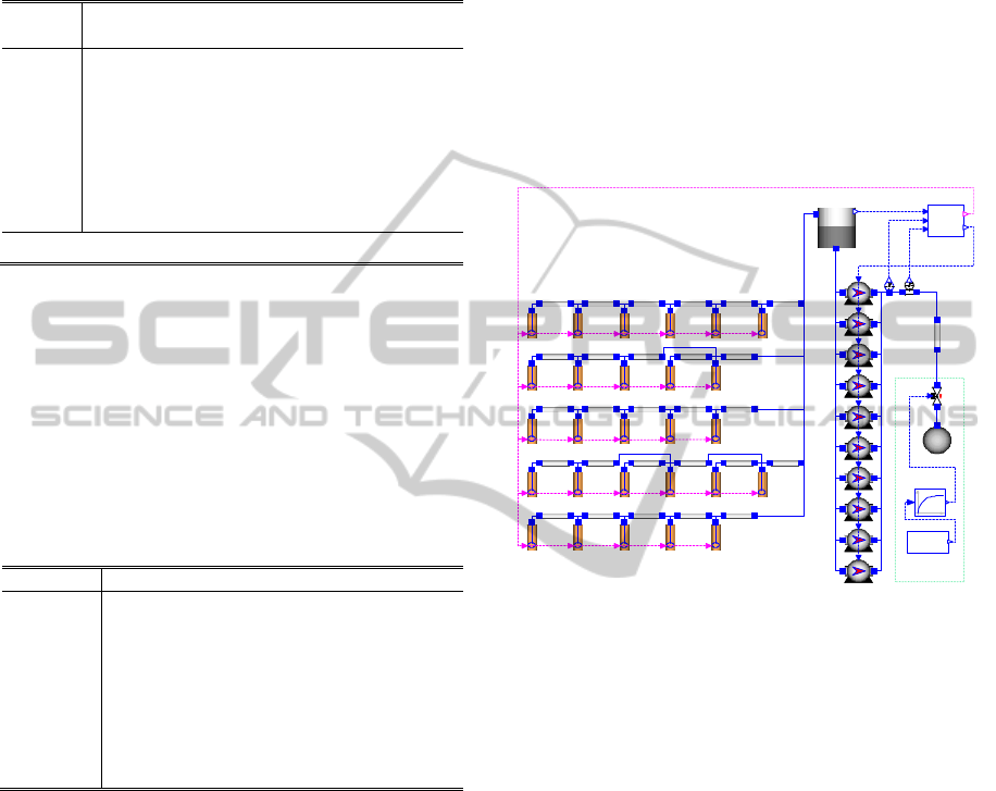
4 SIMULATION RESULTS
The system is built in Dymola and fed by wells’
depths and pipes’ data as illustrated in Figure 10.
Different control schemes and various running
scenarios are examined to validate the model.
Selected results are presented in this section to
provide an overview of the system dynamics.
Figure 10: Top level model of the system.
The control variables are the water level of the
tank (L) and the water flow rate at the distribution
pipe (Q). The tank has a capacity of 8000 m
3
and has
a height of 5m. The reference value of L is set to 4.9
m. This tolerates possible overshoots up to 2% of the
height before occurrence of overflow. Meanwhile, it
utilizes about 98% of storage capacity to handle
possible daily demand variations. The reference
value of the flow is the expected water demand. In
regular conditions, the controller will be able to
manage water distribution as planned. However, in
certain circumstances, the behavior of farmers may
not be as scheduled. This has a direct impact on the
pressure at the distribution network. The controller
should use the pressure signal (P) at the output of the
booster pumps as an interlock variable. The
controller should protect the distribution network
from over-pressure conditions by keeping the signal
P less than the threshold value specified by the
hydraulic system designers (11 bar in our case). On
the other hand, if farmers require more water than
scheduled while having some idle pumping
resources, resultant decrease in the pressure may be
Users
ON/OFF vector
Speed vector
W1 W2 W3 W4 W5
W6 W7 W8 W9 W10 W11
W12 W13 W14 W15 W16
W17 W18 W19 W20 W21
W22 W23 W24 W25 W26 W27
Demand
Rela t iv e
Controller
s
L
P
Q
u
LPF
MODELING, SIMULATION AND CONTROL OF A WATER RECOVERY AND IRRIGATION SYSTEM
327

used by the controller to increase the pumping rate.
However, this has an impact on the aggregated
amount of extracted water. Due to this consequence,
it has been decided to ignore low pressure events so
as to encourage farmers to obey the planned
irrigation schedule.
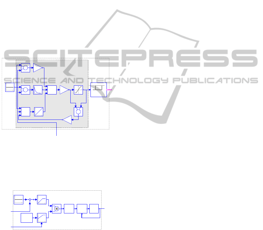
The filling process controller is based on a PID
controller with limited output, anti-windup
compensation and set point weighting as illustrated
in Figure 11 (Astrom, 1995). This PID controller is
available in the Modelica standard library. The
controller is tuned and its output is limited to the
range [0, 25]. The analog output is quantized taking
into account a sufficient hysteresis value (0.4) to
prevent possible oscillations. The resultant number
specifies the required number of running wells. One
should mention that this number is limited to 25 in
order to leave 2 wells as standby.
Figure 11: Filling process controller.
On the other hand, the distribution process has
10 speed-controlled boosters and the maximum
capacity is limited to 8, leaving 2 as standby. The
simulated controller of this process is shown in
Figure 12.
Figure 12: Distribution process controller.
The lower part of the controller has a PID
module with limited output, anti-windup
compensation and set point weighting. Its output
specifies the required pumping capacity which has a
minimum of 0 when all pumps are off and a
maximum of 8·2900 when 8 booster pumps run at
their full speed. The upper part has an integrator
with a limited output [0,1]. In regular cases, the error
signal is positive and the integrator saturates to unity
value. Once the pressure exceeds the specified
threshold (P
th
≈98% of the maximum permissible
pressure), the integrator output starts to decrease and
eventually saturates to 0. This gives a measure for
the persistence of the pressure to exceed the
threshold value. The result of this integrator is
multiplied with the output of the Limited PID
module to generate the recommended pumping
capacity. The distributer module uses this value to
generate the reference speeds for the boosters. In
order to maximize efficiency, only one booster
pump may be assigned a partial load while all others
that share the pumping load must be assigned the
rated speed. The sequencer block regulates the
starting and shutting operations of the boosters. In
order to protect the hydraulic system from water
hummer effects and also to protect the power system
from electrical surges, booster pumps are allowed to
enter or leave operation only one after another.
Having a feedback from the Variable Frequency
Drives (VFD) of the motors, the sequencer is able to
manage that task. The VFD is modeled by a first-
order block with a time constant of 5 s resulting in
an acceleration time of about half a minute to move
forward or backward between zero speed and rated
speed states.
The most important simulation outputs are
shown in Figure 13. The tank’s water level (L) is
depicted in Figure 13a. As intended, the tank starts
at full state in the morning and the controller
returned it back to that state at the end of day. The
number of running pumps, which is shown in Figure
13b, demonstrates how pumps are called for running
when the error signal (deviation from the tank full
state) and its derivative is high in the morning. Later
in the afternoon, supplied water is less than collected
water, and thus the water level in the tank starts to
increase. Consequently, the controller decreases the
number of running pumps. Figure 13c shows the
demanded flow, the scheduled supply flow, and the
supplied flow (Q). The test data is designed to
explore the controller behavior when there is a large
mismatch between demand and scheduled supply.
During the first half of the day, there is excessive
demand and the controller supplies the planned
quantity. In contrast, during the second half of the
day, demand is much less than the scheduled supply.
The controller delivers excess flow to the extent that
pressure (P) at the network does not exceed the safe
limit as illustrated in Figure 13d. Finally, Figure 13e
shows how 6 booster pumps share the pumping load
of that day. At any given time, the controller adjusts
LimPID
L
u
tank's water level
limiter
uMax={25}
limiter
addP
-1
wp
addP
+
wp
-1
addD
-1
wd
addD
+
wd
-1
k={1}
P
I
I
k={16000}
D
k={5000}
k={12}
gainPID
addPID
+1
+1
+1
+
addI
+1
-1
+1
+
addSat
-1
+1
addSat
+
+1
-1
k={0.093}
gainTrack
Quantizer
Setpoint
k={4.9}
P
actual supply flow
speed vector
s
Q
limPID
PID
-
feedback
product
LimIntegrator
I
k={1e-5}
sequenc er
distributer
VFD
Pt h
k={10.8e5}
Supply
Schedualed
ICINCO 2011 - 8th International Conference on Informatics in Control, Automation and Robotics
328

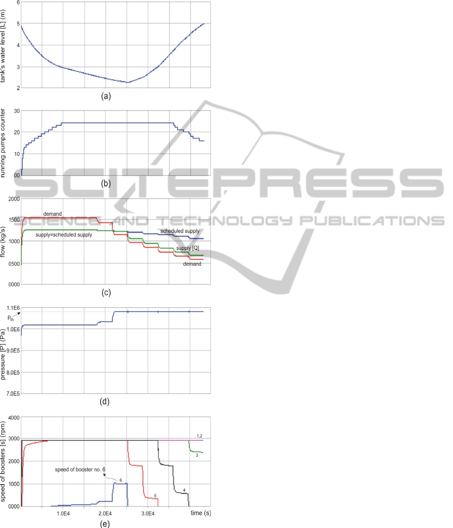
the speed of only one booster pump. Other boosters
are either off or at their rated speed.
Figure 13: Major simulation outputs.
5 SUMMARY AND OUTLOOK
This work presents the design of an easily
manageable model of the water reuse system in
northern Gaza. The resultant model provides a novel
tool for testing the performance of the system under
different operation scenarios and control schemes. It
also helps in understanding the dynamics of the
system and enables designing and tuning a stable
and robust controller for the system. It is our aim in
a future work to elaborate on the control problem
and derive a cost function for running the system. In
other words, we plan to develop a practical criterion
for optimal performance of the system and study the
influence of uncertainties in users’ demand.
ACKNOWLEDGEMENTS
The authors would like to express their gratitude to
Alexander von Humboldt Foundation for supporting
this work. M. Abdelati is also grateful to his
colleagues at The Center for Engineering and
Planning and at the Finnish Consulting Group for
their cooperation.
REFERENCES
Astrom K. and Hagglund T., 1995. PID Controllers:
Theory, Design, and Tuning, North Carolina,
Instrument Society of America, 2nd edition.
Brater E., King H. and Lindell J., 1996. Handbook of
Hydraulics, Mc Graw Hill, New York, 7th Edition.
Elmqvist H., Tummescheit H., and Otter M., 2003.
Object-Oriented Modeling of Thermo-Fluid Systems,
Proceedings of the 3rd International Modelica
Conference, Linköping.
Grundfos, NKG 16 bar End Suction Pumps, pp60: www.
unopomp.com/Resimler/SiteIcerik/NKGendsuctionpu
mps16bar.pdf
Link K., Steuer H., and Butterlin A., 2009. Deficiencies of
Modelica and its simulation environments for
largefluid systems, Proceedings 7th Modelica Confe-
rence, Como, Italy.
Tiller M., 2004. Introduction to Physical Modeling with
Modelica, Kluwer Academic Publishers.
Massachusetts, 2ed printing.
Werner M. et al., 2006. North Gaza Emergency Sewage
Treatment Plant Project - Environmental Assessment
Study, Engineering and Management Consulting
Center.
Ziara M. et al., 2010. Consulting Services for Detailed
Design and Tender Documents of Effluent Recovery
and Irrigation Scheme of NGEST, Joint Venture
Association of the Center for Engineering and
Planning (CEP) and the FCG International Ltd.
MODELING, SIMULATION AND CONTROL OF A WATER RECOVERY AND IRRIGATION SYSTEM
329