DEPLOYMENT OF A WIRELESS SENSOR NETWORK IN

A VINEYARD

José A. Gay-Fernández and Iñigo Cuiñas

Dept. Teoría do Sinal e Comunicacións, Universidade de Vigo, rúa Maxwell, s/n, 36310, Vigo, Spain

Keywords: Propagation, Power decay factor, Wireless sensor network, Vineyard, Node, Sensor, Humidity,

Temperature.

Abstract: A complete analysis for the deployment of a wireless sensor network in a vineyard is presented in this

paper. First, due to the lack of propagation models for peer to peer networks in plantations, propagation

experiments have been carried out to determine the propagation equations. This model was then used for

planning and deploying an actual wireless sensor network. Afterwards, some sensor data are presented and

finally, some general conclusions are extracted from the experiments and presented in the paper.

1 INTRODUCTION

The use of wireless sensor networks is nowadays in

an exponential growing. Initially, these wireless

networks were oriented for indoor use, like home

automation and industrial control (Egan, 2005) or

medical applications (Timmons and Scanlon, 2004).

But many other applications that were not

considered at the beginnings are nowadays coming

to light: outdoor networks and, especially,

sensor/actuator networks in rural areas, forests and

plantations. The research results provided by this

work consider this later environment.

A wireless sensor network is intended to be

deployed in a vineyard, and the maximum distance

between installed nodes is necessary to be

previously estimated. Thus, some propagation

studies have been conducted in order to analyse the

behaviour of such specific radio channel at the

frequency band assigned to these wireless networks:

2.4 GHz. Propagation studies in rural environments

and plantations have to take into account the

presence of vegetation in the propagation channel.

Although there are several research works related to

propagation at such condition (LaGrone and

Chapman, 1961), (Richter, Caldeirinha, Al-Nuaimi,

Seville, Rogers and Savage, 2005) and also an

International Telecommunication Union -

Radiocommunication Sector recommendation [ITU-

R](2007), most of them are focused in classical

master-slave (or base station to mobile terminal)

configuration, where the base has a prominent height

over the coverage area.

However, the proposed sensor application is

intended to be deployed in terms of peer to peer

collaborative networks where both, the transmitter

and the receiver are at similar heights. And there is a

lack in the scientific knowledge for such

configuration (Hashemi, 2008).

Some previous work related to the deployment of

a wireless sensor network (WSN) in a forest has

been checked. Nükhet and Haldun (2009) showed

the importance of these WSN in the forest fire

propagation analysis, but a radio propagation study

appears to be needed in order to optimize the

deployment of these WSN. Hefeeda and Bagheri

(2007) deployed a WSN in order to analyse the

forest fire propagation, but no study was done

regarding the radio propagation conditions in these

wooded environments.

The principal aim of this paper is to provide a

model to estimate the propagation behaviour in

vegetation environments, and to present the results

obtained in an actual wireless network deployment

in a vineyard, installed using this model.

Firstly, a propagation analysis is built, in order to

compute the maximum distances between nodes.

Then, the environment where the WSN were

deployed is presented and after that, the main

elements of the WSN are showed. The following

section indicates the way the network has been

installed. Results regarding sensor data and network

A. Gay-Fernández J. and Cuiñas I..

DEPLOYMENT OF A WIRELESS SENSOR NETWORK IN A VINEYARD.

DOI: 10.5220/0003453100350040

In Proceedings of the International Conference on Wireless Information Networks and Systems (WINSYS-2011), pages 35-40

ISBN: 978-989-8425-73-7

 2011 SCITEPRESS (Science and Technology Publications, Lda.)

behaviour are presented in

the fifth section. Finally,

some conclusions are presented to close this paper.

2 PROPAGATION MODELLING

Before installing the wireless sensor network, it is

necessary to study the maximum distance between

consecutive nodes. There are some propagation

studies in rural environments at 2.4 GHz. Cuiñas,

Gay-Fernandez, Alejos and Sanchez (2010)

presented a study on the propagation in mature

forest at 2.4 GHz. Furthermore, Gay-Fernandez,

Garcia, Cuiñas, Alejos, Sanchez, and Miranda-Sierra

(2010) showed the main parameters to take into

account when deploying a wireless sensor network.

Thus, since wireless sensor nodes were going to be

deployed at a mean height of 3 meters over the

ground, and the vineyard grew up to 2 m, the

propagation environment seems to be quite different

from the ones presented by Cuiñas et. al. (2010).

Since the propagation analysis could not be

performed in a vineyard due to the advanced status

of the vineyard harvest, two measurement

campaigns were deployed into grasslands and

scrublands, in order to obtain a general propagation

equation for the vineyard environment by

extrapolating data from these two different

ambiences.

2.1 Measurement Campaign

A separate transmitter and receiver configuration has

been used during both measurement campaigns.

Thus, large distances between transmitter and

receiver could be accomplished in order to check

how the signal strength attenuation with distance is.

The transmitter equipment consisted of a signal

generator Rohde-Schwarz SMR, which fed an

omnidirectional wide band antenna, Electrometrics

EM-6865. A portable spectrum analyser Rohde-

Schwarz FSH-6 is used at the receiver system with

an omnidirectional antenna, similar to the transmitter

end.

The data was collected around two different

radials at each environment. Each radial consists of

25 points and 150 meters at the grassland

environment, and 16 points and 32 meters at the

scrubland one. The number of power samples

gathered at grass and scrub lands is 301 and 3010

respectively.

Three different heights were analysed for the

transmitting and receiving antennas: 0.9, 1.2 and 1.6

meters. Both antennas were placed at the same

height in our analysis, in order to simulate the best

conditions for a peer to peer propagation.

2.2 Propagation Model

903 power samples per frequency were collected at

each one of the 50 points under measure at the

grassland environment. The power samples per

frequency at each point were 9030 at the scrubland

environment, because there was a high time-variance

of the received power.

The objective of the data processing is the

analysis of the results by means of a regression to

know how the power decays with distance. The

attenuation of the received power seems to fit a

linear equation of the form P=P

-n·10·log

(d),

where d is the distance between transmitter and

receiver in meters, P

is the received power, in dBm,

at 1 meter from the transmitter, P is received power,

in dBm too, at a distance d from the transmitter and

n is a factor that shows the rhythm of the power

decay with distance.

When the previously explained regression fitting

is applied to the collected samples, data from Table I

and II are obtained for grassland and scrubland

respectively. These tables show the attenuation

factors “n

” and “n

”, obtained for the first and

second regression section respectively; the mean

error produced with this estimation; and the cut-off

point of the two regressions. Rows with a dash in

“n

” and “Cut-off point” columns indicate that in

these cases a single regression seems to fit the data

better.

Table 1: Grassland regression data.

H(m) n

Error[dB] Point[m]

0.90 1.75 4.13 1.47 22

1.20 2.07 3.55 1.20 37

1.60 2.04 3.61 1.70 85

Figures 1 and 2 show the equation fitting results

at both environments. All the power values that are

shown in the figures have been normalized to a

transmission power of 0 dBm, in order to easily use

with another transmitting power value.

Table 2: Scrubland regression data.

H(m) n

Error[dB] Point[m]

0.90 2.63 4.63 2.61 13

1.20 2.20 5.18 1.23 13

1.60 1.88 5.58 1.60 13

WINSYS 2011 - International Conference on Wireless Information Networks and Systems

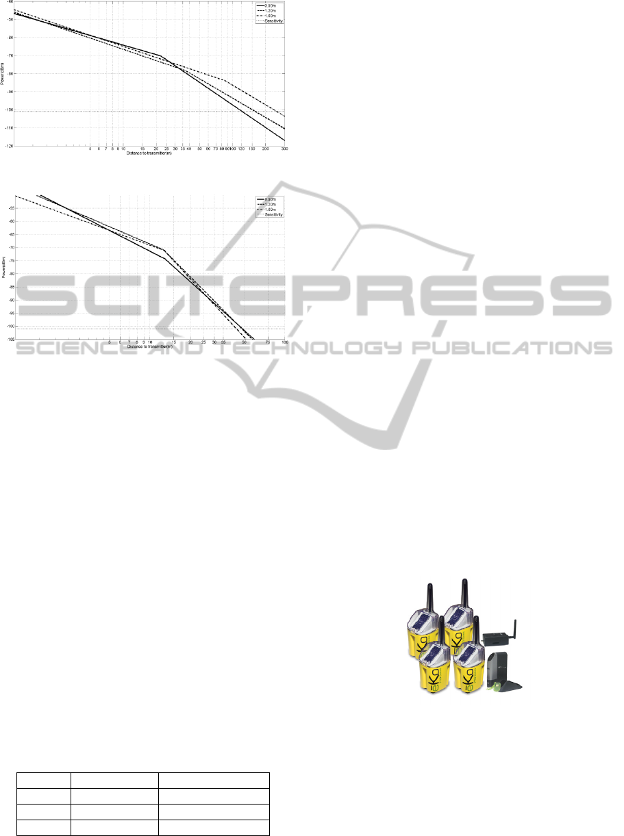
Figure 1: Propagation equations in grasslands.

Figure 2: Propagation equations in scrublands.

2.3 Estimated Distance between Nodes

According to the eko node datasheet, the

transmission power of these wireless nodes is +3

dBm and their sensitivity is -101 dBm. Thus, taking

into account data from tables I and II and these

power values, an estimation of the maximum

distance between nodes could be done for both

environments.

As indicated, figures 1 and 2 show the regression

lines obtained for both environments with the aid of

data from Tables I and II. Furthermore, these figures

show a dotted line at -101 dBm which provides the

maximum range coverage at the point it crosses with

the regression lines. Table 3 shows the maximum

distances between nodes for each

environment and

antenna height. These data have been extracted from

Figures 1 and 2. Thus, when deploying the wireless

sensor network, nodes should be deployed with a

maximum distance of 250 m if there is line of sight

(LoS) between them and at a maximum of 48 meters

if there are scrubs or trees between them.

Table 3: Maximum distances between nodes.

H(m) Grassland Scrubland

0.90 123 m 48 m

1.20 162 m 48 m

160 254 m 44 m

The antenna heights considered for grasslands

and scrublands campaign could represent the

vineyard situation. There, the antennas would be

higher over the ground, but the distance to the

canopies would be similar at these measurements.

3 ENVIRONMENT

The selected environment to deploy this wireless

sensor network is a vineyard located in a mountain

side from Ribadavia, in Ourense, Spain. This

vineyard is property of the winery company

“Vitivinícola del Ribeiro”, a SME founded on the

appellation region “Ribeiro”, in Galicia.

This terrain is located in an exclusive area just in

front of the “Castrelo de Miño” reservoir. The

proximity of such amount of water causes high

humidity in the surrounding terrains, and because of

this, and the high mean temperature, the risk of

suffering a plague in the vineyard rise up to values

extremely high. These are the main reasons for

which this environment has been selected for this

pilot experience.

4 EQUIPMENT

The Crossbow Eko pro series kit was the selected

equipment for the wireless sensor network (WSN)

deployment. This kit is a wireless agricultural and

environmental sensing system for precision

agriculture, microclimate studies and environmental

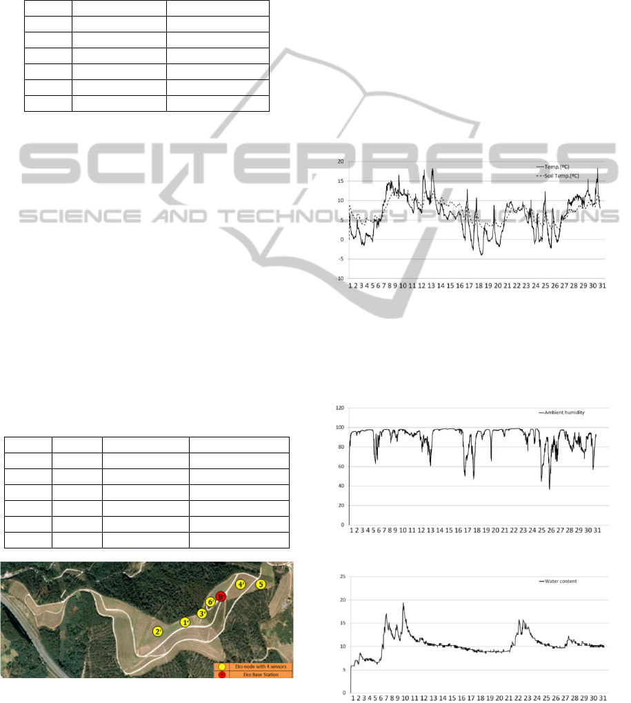
research. Figure 4 depicts the main components of

this WSN kit.

Figure 3: Eko pro series kit.

The Eko system can be enhanced with various

sensors such as soil moisture, ambient humidity and

temperature, leaf wetness, soil water content and

solar radiation. All of them are going to be used in

the deployment under analysis.

The main components of the WSN are showed in

figure 3. There are the eko nodes, an Eko base

DEPLOYMENT OF A WIRELESS SENSOR NETWORK IN A VINEYARD

station, and several sensors plugged into each eko

node. The following sections describe each item in

detail and the way they are interconnected.

4.1 Wireless Sensor Nodes

The eko nodes (Figure 3 in yellow) are a fully

integrated, outdoor, solar-powered wireless sensing

device that allows users to deploy a multi-point

monitoring solution that provides real-time data

from their environment. These nodes are capable of

an outdoor range up to 2 miles depending on the

environment and node hardware configuration

chosen.

Each eko node can accommodate up to 4

different sensors.These nodes integrate a Memsic’s

IRIS processor radio board and antenna, powered by

rechargeable batteries and a solar cell.

Six of these nodes were deployed in this test,

each one with four different sensors plugged in.

4.2 Sensors

Crossbow (2009) contains the main features of the

sensors installed in this pilot. The number of each

kind of sensor in the WSN has been fixed according

to the requirements of the vineyard owner.

4.3 Gateway and Base Station

The eko base station (Figure 3 in black and grey)

consists of three components: the eko base radio, the

eko gateway and the eko view application.

The eko gateway is an embedded sensor network

gateway device. It provides an Ethernet connection

where a PC can be connected to view or copy all the

WSN collected data.

The eko base radio is a fully integrated packaged

that provides the connection between the nodes,

sensors and Gateway. The base radio integrates

another IRIS processor/radio board, antenna and

USB interface board. This interface is used for data

transfer between the base radio and the gateway. The

eko view application has not been used for this pilot,

since data cannot be visualized at the gateway

location.

4.4 WSN Architecture

Sensor data gathered with the aid of the WSN is

going to be locally stored in a PC. Both the

computer and the gateway are going to be installed

in a hut to get power supply for the equipment

during the pilot duration. The location of this hut is

represented as a red circle in Figure 6.

The data stored in the local PC should be

transmitted to a remote server at the University of

Vigo. Thus, all the sensor data could be available in

real time outside the vineyard.

To achieve this data transmission, a GPRS

modem is needed, since there is no line of sight

between the hut location and the winery building.

Figure 4 depicts the main schema of the whole

system.

Figure 4: System Architecture.

Figure 5 shows the transmission system,

composed by the eko base station and a TC-65

GPRS modem from Siemens. This modem is

connected to the laptop by a RS232-serial interface.

5 NETWORK DEPLOYMENT

5.1 Nodes Location

Up to 6 eko nodes have been deployed inside the

Vitivinícola’s vineyard. Each one with four different

sensors plugged in.

The distribution of the nodes along the vineyard

has been done so each one was located in a different

variety of grape, according to the vineyards owner.

Thus, the correspondence between node location and

varietal is shown in table 4. This table depicts also

the estimated distances to the base station.

Figure 5: Transmission System.

According to the recommendations of the

vineyard’s owner, all the eko nodes are able to

measure ambient temperature and humidity, and the

WINSYS 2011 - International Conference on Wireless Information Networks and Systems

same parameters for the soil. Furthermore, the leaf

wetness appears to be quite important, so this sensor

has been connected to each node too. Solar radiation

and soil water content sensors seem to provide less

important data, so they have been equally distributed

within the WSN.

Table 4: Node location and environment.

Node Grape variety Distance to BS (m)

1 Godello 165

2 Albariño 345

3 Treixadura 80

4 Treixadura 200

5 Loureira 295

6 Godello 105

5.2 Network Behaviour

Table 5 shows the final network configuration and

behaviour according to Figure 6 and the data

gathered during December 2010. The second column

presents the following node in the path towards the

base station. These nodes are usually called “father”

node. The third column indicates the distance

between one node and its father. The last column

shows the received signal strength indicator (RSSI)

in dBm between a node and its father. These values

depict that almost all the radio links between one

node and its father are strong. The only one with

some problems is the link between nodes 3 and 6.

This link seems to have very low signal strength

probably because there is a small terrain elevation

between these nodes.

Table 5: Network configuration and behaviour.

Node Father Distance (m) RSSI (dBm)

1 3 88.5 -77.5<P<-74.5

2 1 80 -77.5<P<-74.5

3 6 110 -86.5<P<-83.5

4 Base 156 -77.5<P<-74.5

5 4 150 -77.5<P<-74.5

6 Base 40 -77.5<P<-74.5

Figure 6: Nodes distribution.

The nodes distribution is shown in Figure 6,

where eko nodes are represented as yellow circles,

the base station location is shown with a red circle,

and the Vitivinícola del Ribeiro central building is

represented with a red square.

6 RESULTS

Figures 7 to 10 present different data gathered by the

sensors of the eko nodes.

For instance, Figure 7 shows the evolution of the

ambient and soil temperature, in ºC, during

December, 2010. According to this data, the mean

ambient temperature was 6.28ºC with a standard

deviation of 4.67ºC, while the soil mean temperature

was 7.26ºC with a standard deviation of only 2.63ºC.

Figure 7: Ambient and soil temperature (ºC) Node 2.

Figure 8 represents the ambient humidity of node

7 during the same month. These data reveals that the

mean ambient humidity is around 90% with a

standard deviation of 10%.

Figure 8: Ambient Humidity (%) Node 7.

Figure 9: Soil Water Content (%) Node 7.

DEPLOYMENT OF A WIRELESS SENSOR NETWORK IN A VINEYARD

Figure 9 depicts the soil water content present at

the node 7 location. Peaks at day 7 and 10 indicate

they were rainy days, followed by a 12 days period

almost without rain.

Other sensor data shows, for example, solar

radiation, in Watts per square meter, present at each

node location. (Figure 10).

Figure 10: Solar radiation (W/m

) Node 7.

7 CONCLUSIONS

A complete measurement campaign was developed

to model the propagation channel of the links among

elements of a wireless sensor network. This

propagation model has been used for planning an

actual installation in a vineyard close to Ribadavia,

in Galicia. The Eko technology, from Memsic, has

been selected for this deployment. Up to 6 eko nodes

were set up into the vineyard, to cover an area of

approximately 6 km2.

Four different sensors have been plugged into

each eko node, to collect different ambient and soil

parameters, like humidity, temperature, solar

radiation, water content, etc.

With the aid of these sensor data, vineyard

owners could, for instance, predict the appearance of

a plague in their terrains or optimize the terrain

irrigation. Furthermore, the time between sulphate

applications in the vineyard could be extended. This

last improvement may allow farmers to save a lot of

money in material and labour, and reduce the

amount of chemical products applied to the

vineyard.

ACKNOWLEDGEMENTS

This work has been supported by the Autonomic

Government of Galicia (Xunta de Galicia), Spain,

under Project PGIDIT 08MRU045322PR and by

European Union under project “RFID from Farm to

Fork” (CIP-Pilot actions grant number 250444).

The authors would also like to acknowledge

Manuel Leites, who helped during the deployment.

REFERENCES

Egan, D., April-May 2005. “The emergence of ZigBee in

Building Automation and Industrial Controls”,

Computing & Control Engineering Journal, vol. 16,

no. 2, pp.14-19.

Timmons, N. F. and Scanlon W. G., 2004. “Analysis of

the performance of IEEE 802.15.4 for medical sensor

body area networking," First Annual IEEE

Communications Society Conference on Sensor and

Ad Hoc Communications and Networks, 2004. IEEE

SECON 2004, pp.16-24.

LaGrone, A., Chapman, C., 1961. "Some propagation

characteristics of high UHF signals in the immediate

vicinity of trees," Transactions on Antennas and

Propagation, IRE, vol.9, no.5, pp.487-491.

Richter, J., Caldeirinha, R. F. S., Al-Nuaimi, M.O.,

Seville, A., Rogers, N. C., Savage, N., 2005. "A

generic narrowband model for radiowave propagation

through vegetation," Vehicular Technology

Conference, vol.1, pp. 39- 43

Int. Telecommun. Union (ITU-R), 2007, “Attenuation in

Vegetation,” ITU-R Recomm. 833-6.

Hashemi, H., 2008. “Propagation Channel Modeling for

Ad hoc Networks”, European Microwave Week.

Nükhet S. and Haldun A., 2009. “The Importance of

Using Wireless Sensor Networks for Forest Fire

Sensing and Detection in Turkey”; 5th IATS’09,

Karabuk, Turkey.

Hefeeda, M. and Bagheri, M., 2007."Wireless Sensor

Networks for Early Detection of Forest Fires," IEEE

International Conference on Mobile Adhoc and Sensor

Systems, 2007. MASS 2007, pp.1-6.

Cuinas, I., Gay-Fernandez, J. A., Alejos, A., Sanchez,

Manuel, 2010.”A comparison of radioelectric

propagation in mature forests at wireless network

frequency bands,” European Conference on Antennas

and Propagation (EuCAP), 2010, pp.1-5.

Gay-Fernandez, J. A., Garcia Sanchez, M., Cuiñas, I.,

Alejos, A. V., Sánchez, J. G. and Miranda-Sierra, J.

L., 2010, “Propagation Analysis and Deployment of a

Wireless Sensor Network in a Forest”, Progress In

Electromagnetics Research, PIER 106, pp. 121-145.

Crossbow Technology, Inc, 2009, “Eko PRO Series Users

Manual, Rev. C”.

WINSYS 2011 - International Conference on Wireless Information Networks and Systems