PASSIVITY-BASED NONLINEAR STABILIZING CONTROL
FOR A MOBILE INVERTED PENDULUM
Kazuto Yokoyama and Masaki Takahashi
Keio University, 3-14-1 Hiyoshi, Kohoku-ku, 223-8522, Yokohama, Japan
Keywords: Passivity, Nonlinear Control, Interconnection and Damping Assignment, Mobile Inverted Pendulum,
Experiment.
Abstract: Mobile inverted pendulums (MIPs) need to be stabilized at all times using a reliable control method.
Previous studies were based on a linearized model or feedback linearization. In this study, interconnection
and damping assignment passivity-based control (IDA-PBC) is applied. The IDA-PBC is a nonlinear
control method which has been shown to be powerful in stabilizing underactuated mechanical systems.
Although partial differential equations (PDEs) must be solved to derive the IDA-PBC controller and this is a
difficult task in general, we show that the IDA-PBC controller for the MIP can be derived solving the PDEs.
We also formulate conditions which must be satisfied to guarantee asymptotic stability and show a
procedure to estimate the domain of attraction. Simulation results indicate that the IDA-PBC controller
achieves fast performance theoretically ensuring a large domain of attraction. We also verify its
effectiveness in experiments. In particular control performance under an impulsive disturbance to the MIP
are verified. The IDA-PBC achieves as fast transient performance as a linear-quadratic regulator (LQR). In
addition, we show that even when the pendulum declines quickly and largely because of the disturbance, the
IDA-PBC controller is able to stabilize it whereas the LQR can not.
1 INTRODUCTION
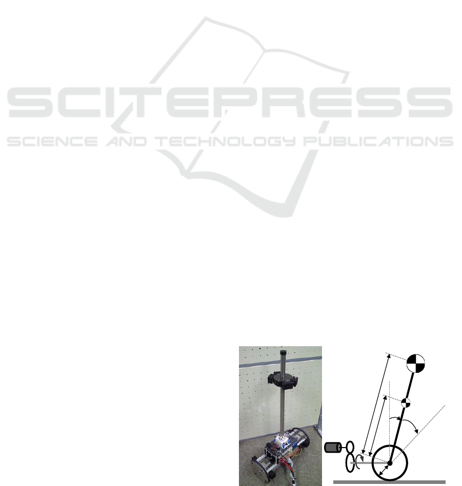
A mobile inverted pendulum (MIP), as shown in
Figure 1, has a small footprint and can turn in a
small radius. The MIP is used as a basic model of
personal mobility devices such as Segway. The MIP
needs to be stabilized at all times using a reliable
control method. Previous studies were based on a
linearized model (Grasser et al., 2002) (Matsumoto
et al., 1993). Other typical approaches use feedback
linearization (Pathak et al., 2005). However, the
former methods can not guarantee stability when the
MIP declines quickly and largely, and the latter ones
require exact parameters of the MIP. These methods
can be inadequate when parameters are uncertain.
In this study we have focused on the MIP in a
two-dimensional sagittal plane in order to design a
nonlinear controller that guarantees large domain of
attraction without using a linearized model or
feedback linearization. This will lead to safe and
reliable operation of the system. For this purpose,
we applied a nonlinear control method called
interconnection and damping assignment
passivity- based control (IDA-PBC) (Ortega et al.,
2002a) to the MIP. This control method shapes the
total energy preserving port-Hamiltonian (PH)
structure (van der schaft, 1999) of the system. Then
stabilization is achieved utilizing passivity of the PH
system.
Passivity is an essential energetic property of
physical systems. In general, control methods
(a) Picture (b) Diagram
Figure 1: The mobile inverted pendulum.
M
w
m
h
m
l
h
l
r
J
w
J
m
J
r
n
r
f
1
q
2
q
τ
128
Yokoyama K. and Takahashi M..
PASSIVITY-BASED NONLINEAR STABILIZING CONTROL FOR A MOBILE INVERTED PENDULUM.
DOI: 10.5220/0003451501280134
In Proceedings of the 8th International Conference on Informatics in Control, Automation and Robotics (ICINCO-2011), pages 128-134
ISBN: 978-989-8425-75-1
Copyright
c
2011 SCITEPRESS (Science and Technology Publications, Lda.)

utilizing passivity are expected to be robust (Ortega
et al., 2001). In addition, the IDA-PBC has been
shown to be powerful in stabilizing underactuated
mechanical systems (Gómez-Estern et al., 2001)
(Ortega et al., 2002b) (Acosta et al., 2005) such as a
cart-inverted pendulum.
To derive the IDA-PBC controller, partial
differential equations (PDEs) must be solved. This is
a difficult task in general. A previous study showed
a constructive solution of the PDEs under several
assumptions and applied the solution to a cart-
inverted pendulum (Acosta et al., 2005). However,
the MIP does not satisfy these assumptions, and thus,
it is still necessary to solve the PDEs.
We show that the PDEs for the MIP can be
solved without using the constructive solution. We
also formulate conditions to guarantee asymptotic
stability and also show a procedure to estimate the
domain of attraction. Although in one study an IDA-
PBC controller was derived for a three-dimensional
MIP, only the pendulum angle was stabilized
(Muralidharan et al., 2009). The stability of the other
states was not considered, and the procedure to solve
the PDEs was different from this study.
The effectiveness of the proposed controller is
verified in simulations and experiments.
2 MODELING
A diagram of the MIP is shown in Figure 1(b). The
physical parameters of the experimental MIP are
shown in Table 1. We ignore the friction and a slip
between the wheel and the ground.
1
q
is the
pendulum angle from the vertical line and
2
q
is the
relative wheel angle with respect to the pendulum
body.
[]
12
T
qq=q
is the generalized position vector
and
g
is the gravity acceleration. Equations of
motion are derived based on a previous study
(Matsumoto et al., 1993). They can be represented as
a PH system (van der schaft, 1999).
2
2
H
u
H
∇
⎡⎤
⎡⎤
⎡⎤ ⎡ ⎤
=+
⎢⎥
⎢⎥
⎢⎥ ⎢ ⎥
∇
−
⎣⎦ ⎣ ⎦
⎣⎦
⎣⎦
q
p
0I
q0
I0
pG
(1)
() () ()
1
1
,
2
T
HV
−
=+
qp p
M
qp q
(2)
11
1
2cos cos
cos 1
aqbaqc
aqc
++
⎡⎤
=
⎢⎥
+
⎣⎦
M
(3)
Table 1: Parameters of the mobile inverted pendulum.
Parameter Unit Value
M
kg
2.3
w
m
kg
0.63
h
m
kg
1.0
J
2
kg m
⋅
-2
1.9 10×
w
J
2
kg m
⋅
-3
1.8 10×
m
J
2
kg m
⋅
-6
2.1 10×
l
m
0.061
h
l
m
0.50
r m
0.075
r
n
- 50
r
f
Nmsrad⋅⋅
0
(
)
11
cosVq e q=
(4)
[]
01
T
=G
(5)
(
)
22
hw wrm
dMmmrJnJ=++ ++
(6)
()
1
hh
aMlmlr
d
=+
(7)
()
{}
22 2
1
hw hh w
bMmmrMlmlJJ
d
=++++++
(8)
()
{}
2
1
hw w
cMmmrJ
d
=+++
(9)
()
hh
g
eMlml
d
=+
(10)
u
d
τ
=
(11)
H
and
V
are the total and potential energy of the
open-loop PH system respectively.
=
p
M
q
is the
generalized momenta. In this study, we consider the
MIP in the upper half plane
()
1
2, 2q
ππ
∈−
.
3 DRIVATION OF CONTROLLER
3.1 IDA-PBC
The IDA-PBC controller for frictionless
underactuated mechanical systems is obtained
solving the PDEs (Ortega et al., 2002b)
(
)
(
)
{
1
1TT
dd
−
⊥−
∇−∇
-1
qq
GpMpMMpMp
(12)
}
1
2
2
d
−
+=JM p 0
{
}
1
dd
VV
⊥−
∇
−∇=
qq
GMM 0
(13)
PASSIVITY-BASED NONLINEAR STABILIZING CONTROL FOR A MOBILE INVERTED PENDULUM
129

where
(
)
2
,
nn×
∈Jqp
is a skew-symmetric matrix,
mn⊥×
∈G is a full rank left annihilator of
G
and
()rank n m
⊥
=−G
.
d
M
and
d
V
are desired inertia
matrix and potential energy of a closed-loop PH
system respectively. Consider we can obtain the
solution of the PDEs, then the IDA-PBC control
input is represented as follows.
es di
=+uu u
(14)
()(
)
1
1
1
2
T
es d d d
HH
−
−
−
=∇−∇+
qq
uGGG MM JMp
(15)
T
di d d
H=− ∇
p
uKG
(16)
es
u
shapes the total energy of the system.
di
u
is
used for achieving asymptotic stability. It is a
negative feedback of the passive output
T
cd
H=∇
p
yG
of the closed-loop PH system and
called damping injection.
0
d
>K
is a constant
matrix.
d
H
is the total energy of the closed-loop PH
system and can be represented replacing
M
and
V
in (2) with
d
M
and
d
V
respectively. The closed-loop
PH system is represented as
1
1
2
d
d
di
d
d
H
H
−
−
∇
⎡⎤
⎡⎤
⎡⎤ ⎡ ⎤
=+
⎢⎥⎢⎥
⎢⎥ ⎢ ⎥
∇
−
⎣⎦ ⎣ ⎦
⎣⎦
⎣⎦
q
p
q0
0MM
u
pG
MM J
(17)
Let
*
q
be a desired equilibrium. If
d
M
is
positive define in the neighbourhood of
*
=
qq
and
(
)
*
arg min
d
V=qq
(18)
is satisfied, then the point
()
*
,q0
is a stable
equilibrium of the closed-loop system with a
Lyapunov function
d
H
. In addition, if the closed-
loop PH system is zero-state detectable, then the
desired equilibrium
()
*
,q0
is asymptotically stable.
3.2 Simplifying PDEs
In this study, a method to simplify the PDEs for a
class of systems (Gómez-Estern et al., 2001) (Ortega
et al., 2002b) is utilized to solve the PDEs and
derive the controller. Three assumptions are required.
Assumption 1:
1mn=−
Under this condition
T
k
⊥
=Ge
and
k
is a natural
number which accounts for the underactuated
coordinate and
k
e
is a vector with all zeros except
the
k
-th element which equals 1.
Assumption 2 and 3:
M
and
d
M
depend only
on the underactuated coordinate respectively.
Under these assumptions, the PDE (12) can be
simplified to ordinary differential equations (ODEs).
()
()
()
()
()
()
1
,1
,
,
1
ddd
k
kk
d
k
kk
dd
dq dq
−
−
⎛⎞
=−
⎜⎟
⎝⎠
MMMM
MM
i
i
(19)
The subscript
(
)
,ij
represents the
i
-
j
element
of the matrix. These ODEs are defined only when
the next condition is satisfied.
(
)
()
(
)
1*
,
0
dk
kk
q
−
≠MM
(20)
3.3 Solutions of PDEs
First, we solve ODEs (19). The assumptions 1 and 2
are clearly satisfied because
2n =
,
1m =
and
1k
=
.
Considering the third assumption, we set
d
M
as
()
(
)
(
)
() ()
11 21
1
21 31
dd
d
dd
mq m q
q
mq mq
⎡
⎤
=
⎢
⎥
⎣
⎦
M
(21)
The ODE is written as (22) and (23)
(
)
(
)
{
}
111 2
1
1
1
2 cos 1 cos
sin
det( )
dd
d
aaqc m aqbcm
dm
q
dq
−− −+ + +−
=
M
(22)
Although the equations of motion of the MIP are
different from those of the cart-inverted pendulum,
the structure of the above ODEs is similar to that of
the previous study (Gómez-Estern et al., 2001).
Focusing on that the right-hand sides of the ODEs
are the first degree with respect to the elements of
d
M
, we set
2d
m
and
3d
m
as
(
)
(
)()
21 21 11dd
mq qmq
α
=
(24)
(
)
(
)()
31 31 11dd
mq qmq
α
=
(25)
2
α
and
3
α
are scalar functions of
1
q
and must be
designed to satisfy the conditions for stability. The
solution of the ODE (22) can be written as
()
()
1
*
1
11
q
q
F
d
dm
mq Ke
μ
μ
∫
=
(26)
()
(
)
{
}
()
21 1
1 1
2cos cos1
sin
det
aaqbcaqc
Fq q
α
−+−−−+
=
M
(27)
where
0
m
K >
is a constant parameter and
*
1
q
is the
desired equilibrium of the pendulum angle and
*
1
0q
=
in this study. In summary, first we design
2d
m
by setting
2
α
, then
3
α
(at the same time
3d
m
) is
obtained from the ODE (23). Therefore, we must
find
2
α
which satisfy the conditions for stability.
Second, we solve the potential energy PDE (13).
The solution of this equation is written as
Φ
is an
arbitrary differentiable function.
Using
d
M
and
d
V
obtained from the above
()
(
)
(
)
(
)
{
}
() ( )
{}
22 2 2 22 2
112 1 1 132 1 1 23
2
1
1
112
2 cos 1 cos 2 cos 2 2 cos 2 cos 2 2
sin
det cos
dd dd d d d
d
dd
a a q c mm a q ac q c c b mm m a q ab q c bcmm
dm
q
dq
maqcm
−+−+−−−+−+++−+
=
−+ +M
(23)
ICINCO 2011 - 8th International Conference on Informatics in Control, Automation and Robotics
130

(a) Body angle (b) Wheel angle (c) Input torque
Figure 2: Regulator performance of IDA-PBC and LQR.
()
()
()
()
() ()
()
1
1
1
0
1,1
1
q
d
d
V
Vdz
q
μμ
μ
−
∂
=+Φ
∂
∫
qq
MM
(28)
()
()
()
()
()
()
()
1
1
1,2
2
1
0
1,1
q
d
d
zq d
μ
μ
μ
−
−
−
∫
MM
q
MM
(29)
procedure, the IDA-PBC control input is calculated
from (14) to (16) where
2
2
2
0
0
j
j
−
⎡⎤
=
⎢⎥
⎣⎦
J
(30)
()
()
()
11
111
22 2
11
1
2
T
dT
dd
dq dq
J
dq dq
−−
⊥−⊥
⎧⎫
⎪⎪
=−
⎨⎬
⎪⎪
⎩⎭
MM
p
GMM G Me
(31)
4 CONDITIONS FOR STABILITY
The IDA-PBC controller is derived by designing
2
α
.
However, we must consider the conditions for
stability and controller performance at the same time.
We formulate
2
α
which satisfies the conditions to
avoid the complex task. We must consider three
conditions:
()
*
1
0
d
q >M
, (18) and (20). The condition
(20) for
d
V
can be interpreted as
(
)
*
0
d
V∇=
q
q
(32)
()
2*
0∇Φ >
q
q
(33)
()
2
*
1
1
2
1
0
d
V
q
q
∂
>
∂
(34)
1d
V
is the first term of
d
V
. The conditions (32) and
(33) are satisfied (Gómez-Estern et al., 2001)
(Acosta et al., 2005) (Ortega et al., 2002b) with
()
()
()
()
{}
2
*
2
P
zzzΦ= −qqq
(35)
where
0P >
is a constant parameter. (34) is
calculated as
()
()
()
1*
1
1,1
10
d
q
−
<MM
and equivalent to
()
*
21
*
1
1
0
cos
q
aqc
α
>>
+
(36)
For simplicity and useful tuning of
2
α
, we set
()
21
112
1
cos
q
q
α
β
β
=
+
(37)
where
1
β
and
2
β
are constants. With this
parameterization and after lengthy calculation, the
all three conditions for stability are represented as
**
2111
cos cosqaqc
ββ
<
−⋅+ +
(38)
*
211
cos q
β
β
>− ⋅
(39)
1
0
β
<
(40)
(
)
()
{
}
()
()
**
11
*
211
2
*
1
2cos cos
cos
cos 2
aqaqbcbc
q
aqc bc
ββ
++ −
<− ⋅ +
++−
(41)
Consequently, if we select
1
β
and
2
β
from the
region characterized by the inequalities, then
*
=
qq
is the isolated minimum of
d
V
and
(
)
*
,
q
0
is stable.
In addition, we can check
0, 0
cdi
yu≡≡
⇒
(
)
(
)
*
,,→qq q 0
with lengthy calculation. Therefore
the desired equilibrium is asymptotically stable at
least in the neighbourhood of
*
11
0qq==
.
An estimate of the domain of attraction can be
calculated evaluating the conditions at general
(
)
1
2, 2q
ππ
∈−
. Although we can not show the
detailed procedure because of the paper space, the
domain can be simply calculated solving
21lim11lim
cos cosqaqc
β
β
=
−⋅+ +
(42)
for
1lim
q
.
d
H
is a radially unbounded function on
the set
(
)
3
1lim 1lim
,qq
−
×
and this is the domain.
5 SIMULATION
The parameters of the IDA-PBC controller are as
follows:
50
m
K
=
,
1
2.3
β
=
−
,
2
4.1
β
=
,
0.35P =
and
45
d
K
=
. The estimate of the domain of attraction is
calculated as
1
0.590q <
. An optimal feedback gain
of the LQR controller is
[
]
303 3.38 65.8 4.26
LQR
=−−−−F
with respect to
a state vector
[]
1212
T
qqqq=x
. These
0 2 4 6 8 10
-0.05
0
0.05
0.1
time
[
s
]
☯
IDA-PBC
LQR
[ra
d
][ra
d
]
0 2 4 6 8 10
-0.05
0
0.05
0.1
time
[
s
]
☯
IDA-PBC
LQR
[ra
d
][ra
d
]
0 2 4 6 8 10
0
0.5
1
1.5
time
[
s
]
☯
IDA-PBC
LQR
[rad][rad]
0 2 4 6 8 10
0
0.5
1
1.5
time
[
s
]
☯
IDA-PBC
LQR
[rad][rad]
0 2 4 6 8 10
-0.5
0
0.5
1
time
[
s
]
☯
IDA-PBC
LQR
[Nm][Nm]
0 2 4 6 8 10
-0.5
0
0.5
1
time
[
s
]
☯
IDA-PBC
LQR
[Nm][Nm]
PASSIVITY-BASED NONLINEAR STABILIZING CONTROL FOR A MOBILE INVERTED PENDULUM
131
parameters are selected by trial and error so that
regulator performance of the controllers are similar
in simulations. Although a large LQR gain will
realize a large domain of attraction, the MIP became
sensitive to sensor noise and we considered it. The
simulation results with the initial state
[]
0
0.1 0 0 0
T
=x
and the desired wheel angle
*
2
0q
=
are shown in Figure 2. Although we can
theoretically design an IDA-PBC controller with a
larger estimate of the domain of attraction such as
1
2q
π
<
, the transient performance tends to be slow.
We utilized knowledge of the trade-off between
performance and the domain (Yokoyama &
Takahashi, 2010) when we tune the IDA-PBC.
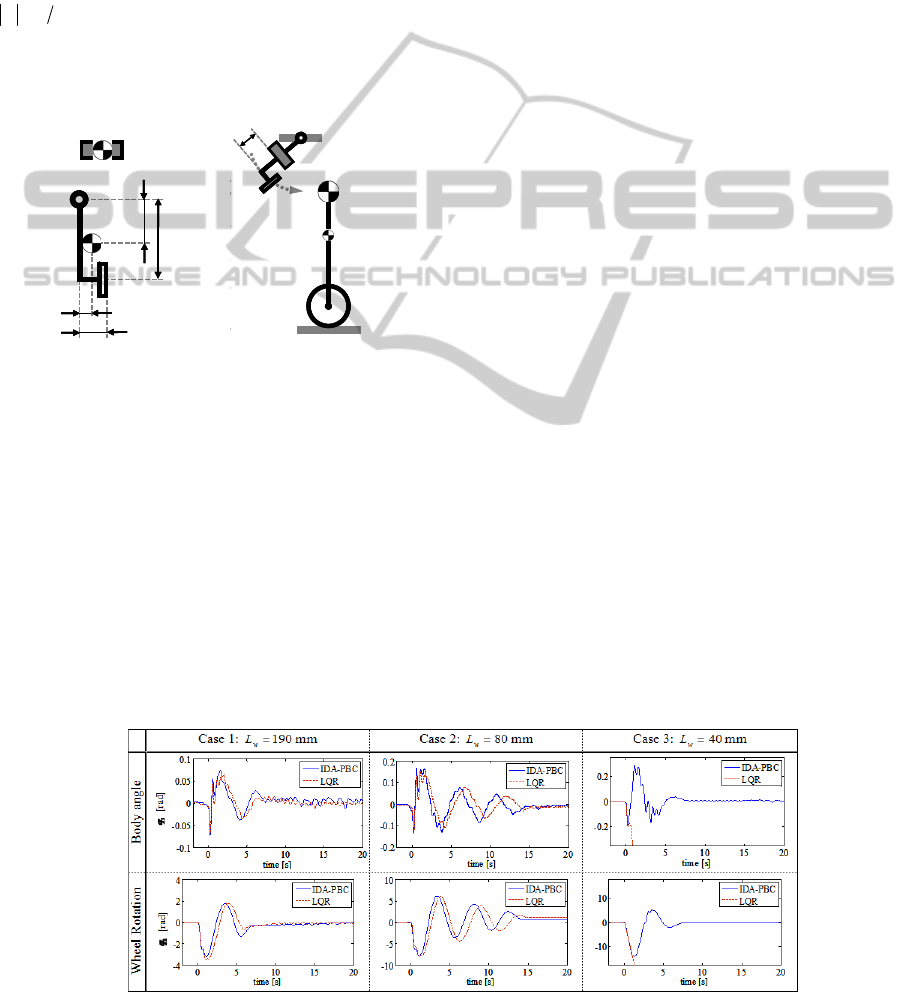
Figure 3: The equipment for adding disturbance.
6 EXPERIMENT
The angular velocity
1
q
was measured with a gyro
sensor, and the angle
1
q
is calculated integrating
1
q
.
We measured angles and angular velocities of the
wheels with encoders, and the average values were
respectively used as
2
q
and
2
q
. An additional
friction compensation torque was added. The friction
was assumed to be Coulomb-type (Matsumoto et al.,
1993). A diagram of the experimental setup is shown
in Figure 3. We added the impulsive disturbance to
the pendulum and compared the performance of the
IDA-PBC and LQR. The disturbance was realized
using an arm hung from a fixed rotational axis. We
lifted the arm to a fixed height and let it go softly,
allowing the arm to collide with the pendulum. We
adjusted the amplitude of the disturbance by
changing
w
L
in Figure 3. The smaller the
w
L
was,
the larger the disturbance became. The experiments
were conducted under three cases of disturbance (
w
L
= 190, 80 and 40 mm); we refer to these as Cases 1,
2 and 3 respectively.
The results are shown in Figure 4. In Case 1, which
corresponds to the smallest disturbance, the both
controllers performed similarly. In Case 2, the IDA-
PBC showed slightly faster performance. In Case 3,
which corresponds to the largest disturbance, only
the IDA-PBC stabilized the MIP. Enlarged time
histories of Case 3 are in Figure 5. Before the yellow
shaded region, both controllers show similar time
histories. However in the region, differences appear
in the pendulum angles and input torque between the
controllers. They gradually expand, and eventually
the MIP with the LQR fell over. The system became
unstable because of the pendulum angle that
declined quickly and largely. Figure 6 shows the
successive pictures of Case 3 with the IDA-PBC.
7 CONCLUSIONS
We have applied the IDA-PBC which is one of the
nonlinear control method based on passivity to
realize a safe stabilizing control of the MIP. The
derivation of the controller depends on the
solvability of the PDEs. We have shown that they
can be solved for the MIP. The derived IDA-PBC
controller does not depend on the linearized model
or feedback linearization. We have also formulated
the conditions for stability and make it systematic to
tune the controller parameters. In simulations, the
Figure 4: Experimental Results.
221 [mm]
150 [mm]
0.148 [kg]
15 [mm]
41 [mm]
0.465 [kg]
221 [mm]
150 [mm]
0.148 [kg]
15 [mm]
41 [mm]
0.465 [kg]
221 [mm]
150 [mm]
0.148 [kg]
15 [mm]
41 [mm]
0.465 [kg]
w
L
221 [mm]
150 [mm]
[kg]
5 [mm]
41 [mm]
g]
w
L
221 [mm]
150 [mm]
[kg]
5 [mm]
41 [mm]
g]
221 [mm]
150 [mm]
[kg]
5 [mm]
41 [mm]
g]
w
L
ICINCO 2011 - 8th International Conference on Informatics in Control, Automation and Robotics
132
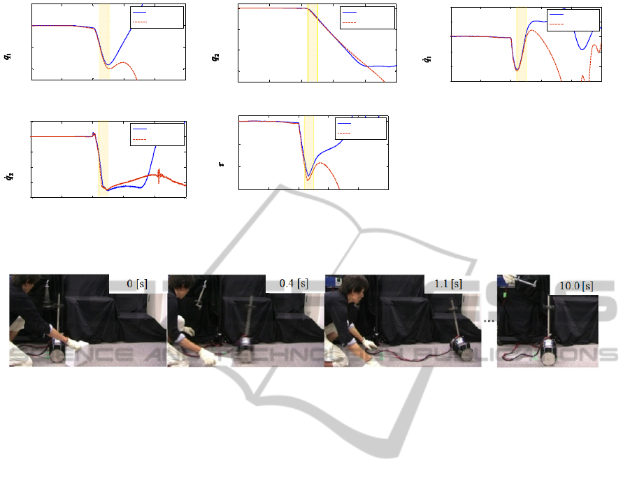
(a) Body angle (b) Wheel angle (c) Body angular velocity
(d) Wheel angular velocity (e) Input Torque
Figure 5: Enlarged Results of The Experiment (Case 3).
Figure 6: The successive pictures of case 3 with the IDA-PBC.
performance of the controller is fast with
theoretically guaranteed large domain of attraction.
The controller has also been applied to the physical
MIP. The impulsive disturbance is added to the
pendulum and the performance of the IDA-PBC is
compared to that of the LQR. Under the small
disturbance, the both show similar performance.
However, when we add the large disturbance and the
MIP goes out of the region where linear
approximation will not be valid, only the IDA-PBC
can stabilize the system. We conclude that the IDA-
PBC controller derived from the nonlinear equations
of motion is superior to the LQR in the physical
application, and effective to stabilize the MIP.
ACKNOWLEDGEMENTS
This work was supported in part by Grant in Aid for
the Global Center of Excellence Program for
"Center for Education and Research of Symbiotic,
Safe and Secure System Design" from the Ministry
of Education, Culture, Sport, and Technology in
Japan.
REFERENCES
Acosta, J. Á., Ortega, R., Astolfi, A. and Mahindrakar, A.
D. (2005). Interconnection and Damping Assignment
Passivity-Based Control of Mechanical Systems with
Underactuation Degree One. IEEE Transactions on
Automatic Control, 50(12), 1936-1955.
Gómez-Estern, F., Ortega, R., Rubio, F. R. and Aracil, J.
(2001). Stabilization of a Class of Underactuated
Mechanical Systems via Total Energy Shaping. IEEE
Conference on Decision and Control, pp. 1137-1143.
Grasser, F., D’Arrigo, A., Colombi, S. and Rufer, A. C.
(2002). JOE: A Mobile, Inverted Pendulum. IEEE
Transactions on Industrial Electronics, 49(1), 107-114.
Matsumoto, O., Kajita, S. and Tani, K. (1993). Estimation
and control of the attitude of a dynamic mobile robot
using internal sensors. Advanced Robotics, 7(2), 159-
178.
Muralidharan, V., Ravichandran, M. T. and Mahindrakar,
A. D. (2009) “Extending Interconnection and
Damping Assignment Passivity-Based Control (IDA-
PBC) to Underactuated Mechanical Systems with
Nonholonomic Pfaffian Constraints: the Mobile
Inverted Pendulum Robot. IEEE Conference on
Decision and Control and Chinese Control
Conference, 6305-6310.
Ortega, R., van der Schaft, A. J., Mareels, I. and Maschke,
B. (2001). Putting Energy Back in Control. IEEE
Control Systems Magazine, 21(2), 18-33.
-1 -0.5 0 0.5 1 1.5
-0.2
-0.1
0
0.1
time [s]
IDA-PBC
LQR
-1 -0.5 0 0.5 1 1.5
-0.2
-0.1
0
0.1
time [s]
IDA-PBC
LQR
[ra
d
][ra
d
]
-1 -0.5 0 0.5 1 1.5
-0.2
-0.1
0
0.1
time [s]
IDA-PBC
LQR
-1 -0.5 0 0.5 1 1.5
-0.2
-0.1
0
0.1
time [s]
IDA-PBC
LQR
[ra
d
][ra
d
]
-1 -0.5 0 0.5 1 1.5
-0.2
-0.1
0
0.1
time [s]
IDA-PBC
LQR
-1 -0.5 0 0.5 1 1.5
-0.2
-0.1
0
0.1
time [s]
IDA-PBC
LQR
[ra
d
][ra
d
]
-1 -0.5 0 0.5 1 1.5
-15
-10
-5
0
time [s]
IDA-PBC
LQR
-1 -0.5 0 0.5 1 1.5
-15
-10
-5
0
time [s]
IDA-PBC
LQR
[rad][rad]
-1 -0.5 0 0.5 1 1.5
-15
-10
-5
0
time [s]
IDA-PBC
LQR
-1 -0.5 0 0.5 1 1.5
-15
-10
-5
0
time [s]
IDA-PBC
LQR
[rad][rad]
-1 -0.5 0 0.5 1 1.5
-15
-10
-5
0
time [s]
IDA-PBC
LQR
-1 -0.5 0 0.5 1 1.5
-15
-10
-5
0
time [s]
IDA-PBC
LQR
[rad][rad]
-1 -0.5 0 0.5 1 1.5
-1.5
-1
-0.5
0
0.5
1
time [s]
IDA-PBC
LQR
-1 -0.5 0 0.5 1 1.5
-1.5
-1
-0.5
0
0.5
1
time [s]
IDA-PBC
LQR
[rad/s][rad/s]
-1 -0.5 0 0.5 1 1.5
-1.5
-1
-0.5
0
0.5
1
time [s]
IDA-PBC
LQR
-1 -0.5 0 0.5 1 1.5
-1.5
-1
-0.5
0
0.5
1
time [s]
IDA-PBC
LQR
[rad/s][rad/s]
-1 -0.5 0 0.5 1 1.5
-1.5
-1
-0.5
0
0.5
1
time [s]
IDA-PBC
LQR
-1 -0.5 0 0.5 1 1.5
-1.5
-1
-0.5
0
0.5
1
time [s]
IDA-PBC
LQR
[rad/s][rad/s]
-1 -0.5 0 0.5 1 1.5
-20
-15
-10
-5
0
5
time [s]
IDA-PBC
LQR
-1 -0.5 0 0.5 1 1.5
-20
-15
-10
-5
0
5
time [s]
IDA-PBC
LQR
[rad/s][rad/s]
-1 -0.5 0 0.5 1 1.5
-20
-15
-10
-5
0
5
time [s]
IDA-PBC
LQR
-1 -0.5 0 0.5 1 1.5
-20
-15
-10
-5
0
5
time [s]
IDA-PBC
LQR
[rad/s][rad/s]
-1 -0.5 0 0.5 1 1.5
-20
-15
-10
-5
0
5
time [s]
IDA-PBC
LQR
-1 -0.5 0 0.5 1 1.5
-20
-15
-10
-5
0
5
time [s]
IDA-PBC
LQR
[rad/s][rad/s]
-1 -0.5 0 0.5 1 1.5
-6
-4
-2
0
time [s]
IDA-PBC
LQR
-1 -0.5 0 0.5 1 1.5
-6
-4
-2
0
time [s]
IDA-PBC
LQR
[Nm][Nm]
-1 -0.5 0 0.5 1 1.5
-6
-4
-2
0
time [s]
IDA-PBC
LQR
-1 -0.5 0 0.5 1 1.5
-6
-4
-2
0
time [s]
IDA-PBC
LQR
[Nm][Nm]
-1 -0.5 0 0.5 1 1.5
-6
-4
-2
0
time [s]
IDA-PBC
LQR
-1 -0.5 0 0.5 1 1.5
-6
-4
-2
0
time [s]
IDA-PBC
LQR
[Nm][Nm]
PASSIVITY-BASED NONLINEAR STABILIZING CONTROL FOR A MOBILE INVERTED PENDULUM
133

Ortega, R., van der Schaft, A. J., Maschke, B. and
Escobar, G. (2002a). Interconnection and Damping
Assignment Passivity-Based Control of Port-
Controlled Hamiltonian Systems. Automatica, 38,
585-596.
Ortega, R., Spong, M. W., Gómez-Estern, F. and
Blankenstein, G. (2002b). Stabilization of a Class of
Underactuated Mechanical Systems via
Interconnection and Damping Assignment. IEEE
Transactions on Automatic Control, 47(8), 1218-1233
Pathak, K., Franch, J. and Agrawal, S. K. (2005). Velocity
and Position Control of a Wheeled Inverted Pendulum
by Partial Feedback Linearization. IEEE Transactions
on Robotics, 21(3), 505-513.
van der Schaft, A. J. (1999). L2-Gain and Passivity
Techniques in Nonlinear Control. Berlin: Springer.
Yokoyama, K. and Takahashi, M. (2010). Stabilization of
a Cart-Inverted Pendulum with Interconnection and
Damping Assignment Passivity-Based Control
Focusing on the Kinetic Energy Shaping. Journal of
System Design and Dynamics, 4(5), 698-71.
ICINCO 2011 - 8th International Conference on Informatics in Control, Automation and Robotics
134
