DESIGN OF A FULLY AUTOMATED ROBOTIC

SPOT-WELDING LINE

M. Selim Akturk, Adnan Tula

Department of Industrial Engineering, Bilkent University, 06800 Bilkent, Ankara, Turkey

Hakan Gultekin

Department of Industrial Engineering, TOBB University of Economics and Technology, 06560 Sogutozu, Ankara, Turkey

Keywords:

Robotic assembly line, Line balancing, Automobile industry.

Abstract:

The mixed model assembly line design problem includes allocating operations to the stations in the robotic

cell and satisfying the demand and cycle time within a desired interval for each model to be produced. We

also ensure that assignability, precedence and tool life constraints are met. Each pair of spot welding tools can

process a certain number of welds and must be replaced at the end of tool life. Tool replacement decisions not

only affect the tooling cost, but also the production rate. Therefore, we determine the number of stations and

allocate the operations into the stations in such a way that tool change periods coincide with the unavailability

periods to eliminate tool change related line stoppages in a mixed model fully automated robotic assembly

line. We provide a mathematical formulation of the problem, and propose a heuristic algorithm.

1 INTRODUCTION

This study focuses on a robotic cell mixed-model

assembly line design problem in which automotive

body components are produced. The problem is to de-

termine the number of stations to be established, to al-

locate the welding operations to these stations with a

constraint on the cycle time and, different from the lit-

erature, to determine the tool change periods in order

to maximize the total proﬁt. Each station consists of

a single robot equipped with spot welding guns. Each

gun has spot welding tools used to perform welding

operations. These tools have limited life time which

is represented by the total number of spot welds that

they can process.

Numerous studies have been conducted by re-

searchers, in which different aspects of assembly line

design problems are considered such as the layout of

the line, equipment selection and line balancing. The

interested reader can see the recent surveys by Becker

and Scholl (2006) and Boysen et al. (2007). In this

study, different from the existing ones, we address

a mixed-model assembly line problem with a proﬁt

maximizing objective. We aim to determine the num-

ber of stations to install, which effects the station in-

stallation costs and the throughput rate; the assignme-

nt of operations to the stations, which effects through-

put rate and tool usage (as a consequence the tool-

ing cost); and tool change periods, which effect cycle

time and tooling costs. Therefore, the relevant terms

for the total proﬁt function are the individual proﬁts

from each manufactured component (revenue minus

all the costs except the tooling and station installa-

tion costs), tooling cost, and station installation cost.

As a consequence, we deﬁne the total proﬁt function

as the difference between the sum of individual prof-

its gained by manufacturing components of the ﬁnal

products and the sum of investment costs for stations

and tooling. Station investment costs include robot,

ﬁxture and space costs. Tooling costs are incurred

over time as the tools are replaced with new ones.

Prior studies do not consider the unavailability peri-

ods of assembly lines and assume that assembly lines

work 24 hours a day continuously. In this study, we

take such breaks into account to reﬂect a more realis-

tic production environment.

In Gultekin et al. (2006), we dealt with the robotic

cell scheduling problem with two identical CNC ma-

chines and a single material handling robot. We al-

ready showed that the previous theoretical results on

the same problem were no longer valid when we

added the tool life related constraints to the problem

387

Selim Akturk M., Tula A. and Gultekin H..

DESIGN OF A FULLY AUTOMATED ROBOTIC SPOT-WELDING LINE.

DOI: 10.5220/0003442603870392

In Proceedings of the 8th International Conference on Informatics in Control, Automation and Robotics (ICINCO-2011), pages 387-392

ISBN: 978-989-8425-75-1

 2011 SCITEPRESS (Science and Technology Publications, Lda.)

setting since the cycle times depend on the allocation

of the operations. Tool life has a number of implica-

tions in the current problem setting as well: Contin-

uing to use a tool even after its life is over results in

quality problems and, thus, the tools must be replaced

before their lives end. On the other hand, replacing a

tool before its life is over increases the tooling cost.

Additionally, the life of a tool may end at a time in-

stance when the assembly line is supposed to be op-

erating and therefore may result in line stoppages. In

order to overcome this problem, we aim to design the

line so that the tools are changed in periods of un-

availability in which the line is already not operating.

At each break, if there exist welding tools that have

a remaining number of spot welds less than the total

number of spot welds that they have to perform until

the next break, they must be replaced with new ones.

With such an operating rule and by assigning the op-

erations to the stations considering not only the cycle

times but also the tool usage rates at each station, we

prove that the total proﬁt can be increased.

The design problem that we study in this paper is

originated from a project that we conducted for one

of the leading automotive manufacturing companies

in Turkey. One of the important aspects of any design

problem is the operational problems that can be faced

during the actual implementation of the design. We

ﬁrst investigated the existing automotive body com-

ponent robotic spot welding assembly line, where the

line is fully automated to produce two models in any

order. In that project, our aim was to develop a tool

change decision policy for the assembly line where

there was no systematic approach for scheduling the

tool change periods. All of the tools were being re-

placed just at the end of their lives. As a consequence,

the line was stopped regularly for tool changes. The

company has allocated almost 10% of their available

capacity to the line stoppages due to tool changes.

This is the main reason why we study line design

and operation allocation problems together with the

scheduling of tool change periods in this study.

2 PROBLEM DEFINITION

We consider an assembly line that contains at most

m stations: S

, j ∈ M={1, 2,. .., m}. Space restric-

tions in the production area and a limited budget for

investment costs are among the reasons of such a re-

striction on the number of stations. We use parameter

to denote the cost of setting up S

. There are g dif-

ferent models to be produced in this robotic assembly

line. O

represents operation i of a part of model h;

i ∈ N

= {1, 2, . . . , n

}, h ∈ G = {1, 2, . . . , g}. A num-

ber of spot welds are grouped together to form an op-

eration. The selection is based on the closeness of

the welds to each other and to satisfy the proper ge-

ometry of the assembled components. Let W

be the

number of spot welds required to perform operation i

on model h. The total number of spot welds that the

welding tool in S

can process before its life is over is

denoted by B

Factors that affect the number of stations to be

installed are the target cycle time, the station invest-

ment cost, and the tooling cost. Let us represent the

yearly expected demand for the parts to be produced

as θ

. We use the parameter γ

to denote the target

cycle time for model h to meet the yearly expected

demand θ

. In general, let T

be the total time allo-

cated for production of model h; f

the actual cycle

time of model h; and

the corresponding production

quantity. Then, we have the following:

∀h.

Producing model h less than a speciﬁed quantity is

not acceptable. Let this speciﬁed quantity be denoted

by θ

and the corresponding cycle time be denoted by

, which speciﬁes an upper bound on the cycle time.

Additionally, if production exceeds a certain quantity

for each model, it is not possible to make any addi-

tional proﬁt. Let this production level be denoted by

and the corresponding cycle time lower bound be

denoted by γ

. Clearly, we have θ

≤ θ

. Ad-

ditionally, the individual proﬁt gained from model h

is assumed to be a piecewise linear function. It is de-

noted by PR

for

≤ θ

. On the other hand, if the ac-

tual production amount of model h exceeds the yearly

demand of θ

so that θ

≤ θ

, then the proﬁt

for each model h produced as surplus is PR

, where

= PR

− ∆

, 0 ≤ ∆

≤ PR

, where ∆

denotes

the reduction in the individual proﬁt for the excess

parts when the production exceeds the expected de-

mand. As a consequence, the individual proﬁts from

each model h is a two-piece linear function where the

slope of the second piece is less than that of ﬁrst piece.

In this study, we consider the tool change periods

as a decision variable. If the tools are only changed

at scheduled breaks as we propose, the line will never

stop for a tool change, which increases the throughput

rate, but on the other hand, some tools will be changed

before their lifetime ends. Therefore, the tooling cost

will be increased. As a result, one aim of the current

study is to determine the best solution that balances

the increased tooling cost with the increased through-

put rate. Let C

be the cost of the tools in S

. We as-

sume there are q = 1, 2, . . . ,U, total number of breaks

in the planning horizon. We also need the following

decision variable:

= Binary variable indicating whether tools in S

are changed in tool change period q or not.

ICINCO 2011 - 8th International Conference on Informatics in Control, Automation and Robotics

388

A huge number of spot welds is required to com-

plete the production of a part. Depending on the lo-

cation of these welds and the geometry of the parts, it

may not be possible for a particular type of welding

gun to reach every location on a part and the special

characteristics of the weld such as the diameter and

the thickness may require a different welding tool.

Hence, several types of guns and tools can be loaded

on the robots and hence we need the following param-

eter indicating the assignability of operations.

hij

= 1, if operation i of model h is assignable to S

;

0, otherwise.

Additionally, we have a precedence relation

among the operations which is indicated with the fol-

lowing parameter:

hik

= 1, if operation i precedes operation k in model h;

0, otherwise.

Let t

be the time required to perform operation

i of model h. We calculate t

as a function of the

number of spot welds required to perform operation i

of model h as follows: t

= α+ β ·W

∀h, i, where

α is a constant that denotes the time required for the

robot to reach to the location to perform operation i of

model h and β is another constant that corresponds to

the time required to process a single spot weld.

We deﬁne the parameter ψ

as the ratio of the total

yearly required time to process all demanded parts of

model h to total yearly required time to process all

demanded parts of all models. This ratio is the time

allocated for production of parts of model h and can

be calculated as follows:

· γ

∑

l=1

· γ

∀h.

In most automotive companies (including the one

with which we have been collaborating), the produc-

tion time between two breaks is equal and lasts 6300

seconds within a shift. In order to calculate the re-

maining tool life at each break we need to calculate

the time allocated for the production of parts of all

models between two breaks as 6300· ψ

seconds.

In addition to z

, the other decision variables that

we will use to formulate our model are deﬁned below:

= remaining number of spot welds that the tool

in S

can process after tool change period q.

= actual cycle time for model h.

= 1, if S

is used in the assembly line; and 0, o.w.

hij

= 1, if operation i of model h is assigned to sta-

tion j; and 0, o.w.

The nonlinear mixed-integer mathematical model

can be formulated as follows:

Model 1 (NLMIP):

Max

∑

h=1

· min{

· γ

, θ

}

∑

h=1

· min{max{

· γ

− θ

, 0},

· γ

− θ

}

− ρ·

∑

j=1

∑

q=1

· z

− η·

∑

j=1

· σ

(1)

Subject to

≥ τ

∑

i=1

· x

hij

∀h, j (2)

≤ γ

∀h (3)

hij

≤ a

hij

· σ

∀h, i, j (4)

∑

j=1

hij

= 1 ∀h, i (5)

hik

∑

l=1

hil

+ (1− p

hik

) ≥ x

hk j

∀h, i, j, k (6)

= B

· z

+ [R

j(q−1)

−

∑

h=1

6300· ψ

∑

i=1

· x

hij

](1−z

) ∀ j, q (7)

= B

∀ j (8)

≥

∑

h=1

6300· ψ

· (

∑

i=1

· x

hij

) ∀ j, q (9)

≥ 0, R

≥ 0, x

hij

, σ

, z

∈ {0, 1} ∀h, i, j, q (10)

The objective function is a piecewise linear func-

tion that includes the individual proﬁts that can be

earned by producing up to θ

parts of model h and

the reduced proﬁts for the situation of producing more

than θ

as well as the tooling and station investment

costs. Tooling and station costs are converted to an-

nual costs by the constants ρ and η, which depend

on the selection of the total number of tool change

periods in the planning horizon, U, and the number

of months that the production of the selected models

will continue, respectively. Constraint (2) ensures that

the cycle time is the maximum station time, which is

the sum of the operation times allocated to that sta-

tion plus a constant τ

required for the robot in station

j to begin and ﬁnalize processing the allocated oper-

ations. (3) prevents the actual cycle time for model

h from exceeding γ

. Constraint (4) restricts opera-

tions to be assigned only to the stations where they

can be performed and to stations which are used in

the assembly line. By (5), we ensure that an opera-

tion is assigned to exactly one station and none of the

operations remain unassigned. Constraint (6) allows

an operation to be assigned to a station if all its pre-

decessor operations are assigned to the same or to a

preceding station. Constraint (7) is a coupling con-

straint that connects different product models to com-

pete for a limited tool life at each station. It also han-

dles updates for the remaining number of spot welds

DESIGN OF A FULLY AUTOMATED ROBOTIC SPOT-WELDING LINE

389

for welding tools. If the tool is replaced at that tool

change period, the life time of the tool is reset. Oth-

erwise, the remaining tool life is calculated by sub-

tracting the number of spot welds performed during

the last working period from the tool life at the begin-

ning of this working period. The lifetimes of the tools

are initialized in Constraint (8). By constraint (9), we

guarantee that none of the welding tools ﬁnishes its

lifetime between two breaks.

This is a nonlinear mixed integer programming

formulation. We could use DICOPT, a nonlinear

solver included in GAMS software, to solve this

formulation. Initial tests proved that this nonlinear

model is not efﬁcient in solving the problem.

3 LINEARIZATION OF NLMIP

In this section we present the methodology for lin-

earization of Model 1. We will linearize the objec-

tive function (e.g., Equation (1)), Constraints (2), (3),

(7), and (9) of NLMIP with some well-known tech-

niques. First, we replace

, which frequently occurs

in Model 1 with a new variable ω

. As a result, the

piecewise linear proﬁt part of the objective function

becomes

∑

h=1

· min{θ

· γ

· ω

, θ

}

∑

h=1

· min{max{θ

· γ

· ω

− θ

, 0},

· γ

−θ

}

In order to linearize this we introduce newpositive

variables AO

, λ

, BO

and a binary variable y

The new objective function can be written as follows:

∑

h=1

· AO

∑

h=1

· BO

− ρ ·

∑

j=1

∑

q=1

· z

−η·

∑

j=1

· σ

We also require the following constraints:

≤ θ

· γ

· ω

∀h (1.1)

≤ θ

∀h (1.2)

· γ

· ω

− θ

= λ

− λ

∀h (1.3)

≤ F · y

∀h (1.4)

≤ F · (1− y

) ∀h (1.5)

≤ λ

∀h (1.6)

≤

· γ

− θ

∀h (1.7)

Proposition 1. Constraints (1.1)-(1.7) correctly lin-

earize the objective function of Model 1 given in

Equation (1).

Replacing ω

, e

hij

= x

hij

· ω

, and using a

very large number F, Constraint (2) can be replaced

by the following linear constraints:

hij

≤ ω

∀h, i, j (2.1)

hij

≤ F · x

hij

∀h, i, j (2.2)

hij

≥ ω

− F ·(1− x

hij

) ∀h, i, j (2.3)

hij

≥ 0 ∀h, i, j (2.4)

1 ≥ τ

· ω

∑

i=1

· e

hij

∀h, j (2.5)

Proposition 2. Constraints (2.1)-(2.5) correctly lin-

earize Constraint (2).

Since ω

is strictly positive, Constraint (3) can be

rewritten as follows:

· ω

≥ 1 ∀h. (3.1)

Whereas Constraint (7) can be replaced with the fol-

lowing linear constraints:

≤ R

j(q−1)

∀ j, q (7.1)

≤ F · z

∀ j, q (7.2)

≥ R

j(q−1)

− F ·(1− z

) ∀ j, q (7.3)

≥ 0 ∀ j, q (7.4)

hijq

≤ e

hij

∀i, j, q (7.5)

hijq

≤ F · z

∀i, j, q (7.6)

hijq

≥ e

hij

− F ·(1− z

) ∀i, j, q (7.7)

hijq

≥ 0 ∀i, j, q (7.8)

= B

· z

+ R

j(q−1)

− O

−

∑

h=1

6300· ψ

· (

∑

i=1

· e

hij

)

∑

h=1

6300· ψ

· (

∑

i=1

· π

hijq

) ∀ j, q (7.9)

Proposition 3. Constraints (7.1)-(7.9) correctly lin-

earize Constraint (7). Replacing e

hij

= x

hij

· ω

as in

Constraint (7) also linearizes Constraint (9):

ICINCO 2011 - 8th International Conference on Informatics in Control, Automation and Robotics

390

≥

∑

h=1

6300· ψ

· (

∑

i=1

· e

hij

) ∀ j, q. (9.1)

Having linearized the objective function and the

necessary constraints, we ﬁnally have the following

mixed integer model(MIP):

Max

∑

h=1

· AO

∑

h=1

· BO

− ρ·

∑

j=1

∑

q=1

· z

− η·

∑

j=1

· σ

S.t. Constraints (1.1)-(1.7)

Constraints (2.1)-(2.5)

Constraint (3.1)

Constraints (4)-(6)

Constraints (7.1)-(7.9)

Constraint (8)

Constraint (9.1)

Constraint (10)

, AO

, BO

, λ

, R

≥ 0, y

∈ {0, 1} ∀h, i, j, q

This MIP formulation can be solved using any

commercial LP solver. However, for large scale prob-

lems, in order to get solutions in reasonable times we

also developed a two-stage heuristic algorithm. The

ﬁrst stage of this algorithm ﬁnds a set of feasible so-

lutions for a given γ

value and the second stage is

an improvement algorithm to obtain stronger results

from the given initial feasible solutions.

Example. An automotive company is planning to

set up a robotic cell assembly line to produce body

components for two different models of cars. Next

year, the company plans to sell 150000 cars of the

ﬁrst model and 75000 cars of the second model. To

achieve this production amount, the company sets a

target cycle time of 76 seconds for both models. In or-

der to meet the orders received so far, a cycle time of

at most 80 seconds should be satisﬁed for both mod-

els. Market research shows that the company can not

sell cars more than the amount that can be produced

when the cycle time is 60 seconds for both models.

Cost analysis shows that up to the production amount

of 150000 for the ﬁrst model and 75000 for the sec-

ond model, each body component produced will con-

tribute a proﬁt of $10. In case of producing more than

the expected demand, each excess body component

produced will contribute an expected proﬁt of $7 for

both models. In the production area, there is avail-

able space for at most ten stations. The cost of setting

up one station in the assembly line is $192500. The

welding tools have a tool life of 3200 spot welds and

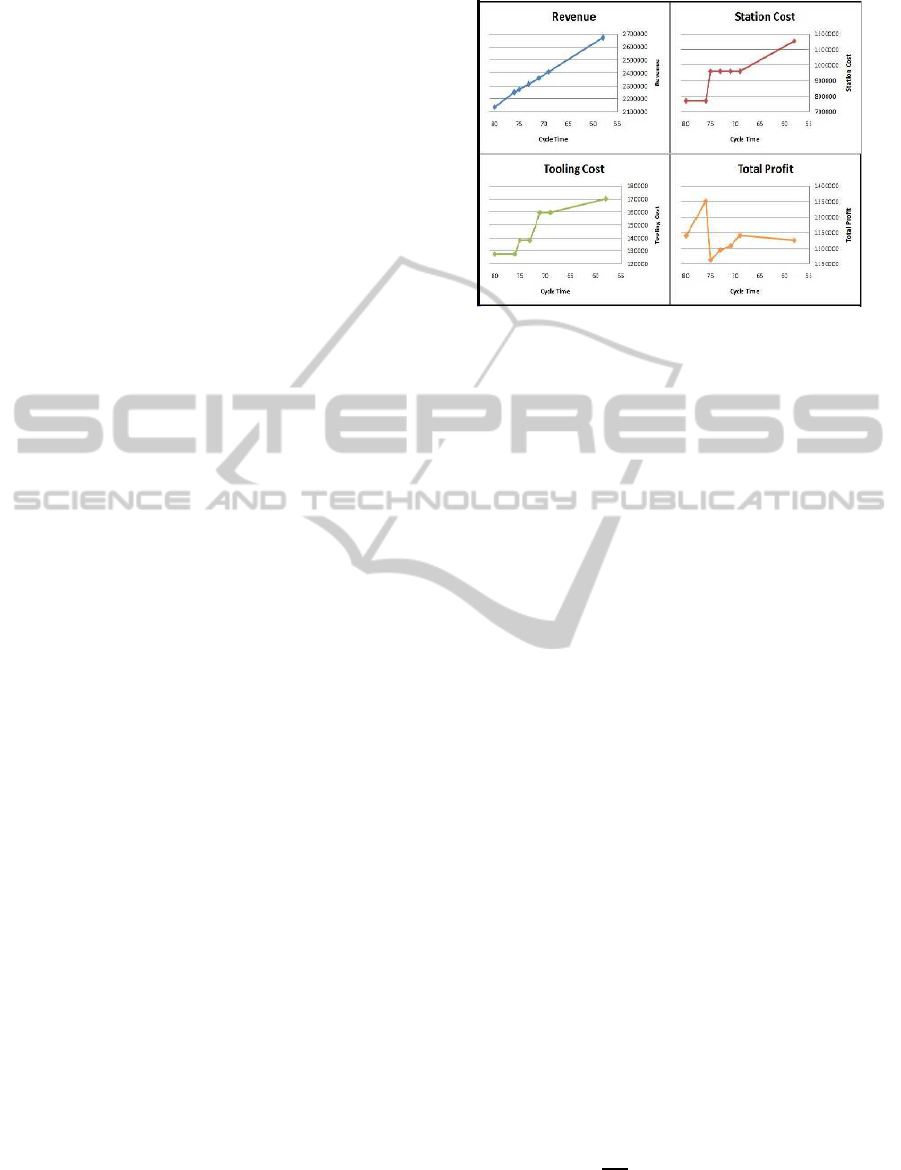
Figure 1: Cost and Proﬁt Values for Example 1.

each welding tool costs $10. Both models require 15

spot welding operations and the number of spot welds

required to perform these operations are 10, 8, 8, 7,

10, 9, 8, 7, 10, 9, 7, 6, 13, 12 and 10, respectively.

The time required for a robot in a station to reach to

the position to perform an operation, the time required

to performa single spot weld and the time required for

a robot to begin and ﬁnalize processing the allocated

operations are calculated to be 1, 2 and 3 seconds,

respectively. Figure 1 depicts the components of the

objective function one at a time as well as the total

proﬁt with respect to the cycle time. As seen in this

ﬁgure, revenue, which is the sum of the proﬁts that

each product contributes, strictly increases as the cy-

cle times decrease, until to γ

values. Station cost is

a nondecreasing function as the cycle times decrease

because lower cycle times require larger number of

stations and it exhibits a stepping structure due to the

breakpoints that correspond to particular cycle times.

4 COMPUTATIONAL STUDY

In this section, we will evaluate the performances of

the proposed heuristic algorithm and the mathemati-

cal formulations (CPLEX version 10.1 is used as the

MIP solver). There are two important factors that af-

fect the size of our problem and optimal allocations

in the solutions. The ﬁrst one is the number of dif-

ferent models that will be produced in the robotic cell

assembly line, denoted as g. As this parameter in-

creases, our problem becomes harder to be solved by

the CPLEX. The second one is the ratio of the proﬁt

contribution of the models to the station investment

cost, denoted as

. This ratio is very important

to evaluate the tradeoff between the revenue and the

number of stations that will be used in the assembly

line. We set two levels as low and high for both of

DESIGN OF A FULLY AUTOMATED ROBOTIC SPOT-WELDING LINE

391

these factors. For the number of models g = 2 is used

for the low and g = 4 is used for the high levels. The

cost of setting up one station is a constant and selected

asV

= 180000 for j = 1, 2, . . . , m. When the ratio

is at its low level, PR

is a uniform random number

from the interval [5,7]. When this ratio is at its high

level, this interval is changed to [9,11]. We take 5

replications for each combination resulting in 20 dif-

ferent randomly generated runs.

The value of the parameter n

, the number of spot

welding operations required for model h, is a uni-

form random number from the interval [8,15]. The

value of the parameter W

, the number of spot welds

required to perform operation i of model h, is also

a uniform random number from the interval [6,15].

When the number of models is at the low level, we

use θ

= 150000 and θ

= 75000 and at the high level,

we use θ

= 100000, θ

= 50000, θ

= 50000 and

= 25000 for the values of expected demands. We

set the value of the expected proﬁt for each excess

production of model h as PR

= ⌈PR

·0.7⌉. An oper-

ation can be allocated to any station. The precedence

relationship matrix is not included due to space limi-

tations, but can be obtained from the authors.

We now continue with some numerical results of

our computationalstudy. First, we solve each run with

the ﬁrst stage of our algorithm which ﬁnds a set of

feasible solutions. Then we use these solutions as ini-

tial feasible solutions for both the MIP model and the

second stage of our heuristic which is the improve-

ment step. The reason that we insert initial solutions

to CPLEX is to improve the quality of the solutions.

Table 1 summarizes the results. Note that, since the

CPLEX runs are terminated after a time limit of 2

hours, the proposed algorithm provided better results

than the CPLEX for all runs.

5 CONCLUSIONS

In this study, we considered a mixed-model assembly

line design problem with the objective of maximizing

the total proﬁt. We considered unavailability periods

and ﬁnite tool lives. We ﬁrst formulated the problem

as an NLMIP model and then provided the linearized

MIP version of it. We also developed a heuristic algo-

rithm that obtains a set of feasible solutions and im-

proved these solutions by incorporating a surrogate

problem. The results of the computational study in-

dicate that this heuristic is very efﬁcient in terms of

CPU time and the quality of the solutions found in

comparison to CPLEX. Our study is the ﬁrst one to

consider unavailability periods and tool changes in

the assembly lines, and to eliminate the tool change

Table 1: Total Proﬁt Values and CPU Times.

Algorithm Best Possible MIP

Run # Algorithm CPU Time MIP (for MIP) CPU Time

1 507340 3.5 478044 792832 7200

2 557526 2.7 536910 760823 7200

3 699150 5.6 699150 943616 7200

4 399544 3 354909 687143 7200

5 622650 3.8 583862 951209 7200

6 1493919 2.8 1465125 1754679 7200

7 1339032 2.7 1312737 1568786 7200

8 1509570 2.3 1401586 1718384 7200

9 1321299 4 1321299 1615406 7200

10 1882792 2.2 1882792 2117928 7200

11 713824 8.4 668407 957151 7200

12 583417 13.4 478329 809448 7200

13 453502 262.6 401048 846789 7200

14 634184 7.1 586373 894127 7200

15 723984 14.6 657755 954369 7200

16 1558088 4.2 1516720 1783367 7200

17 1725291 8.4 1663509 1999991 7200

18 1272524 32.9 1200298 1598373 7200

19 1130496 363.3 1042092 1460130 7200

20 1210876 214.6 1205923 1549724 7200

related line stoppages. For future research, ﬂexibility

can be inserted to the scope of our study by consid-

ering controllable processing times instead of using

deterministic processing times for the assembly line

operations as discussed in Gultekin et al. (2008).

ACKNOWLEDGEMENTS

This research was partially supported by TOFAS¸ T¨urk

Otomobil Fabrikası A.S¸. (Fiat Turkey). We would

like to thank Dr. Orhan Alankus¸, Koc¸ Holding,

Strategic Planning Group, Technology and Environ-

ment Coordinator, and TOFAS¸, Production Technol-

ogy Department, for their continual support.

REFERENCES

Becker, C. and Scholl, A. (2006) A survey on problems and

methods in generalized assembly line balancing. Eu-

ropean Journal of Operational Research, 168, 694-

715.

Boysen, N., Fliedner, M. and Scholl, A. (2007) A classiﬁ-

cation of assembly line balancing problems. European

Journal of Operational Research, 183, 674-693.

Gultekin, H., Akturk, M. S. and Karasan, O. (2006) Cy-

cling scheduling of a 2-machine robotic cell with tool-

ing constraints. European Journal of Operational Re-

search, 174, 777-796.

Gultekin, H., Akturk, M. S. and Karasan, O. (2008) Bicrite-

ria robotic cell scheduling. Journal of Scheduling, 11,

457-473.

ICINCO 2011 - 8th International Conference on Informatics in Control, Automation and Robotics

392