
A NEW METHOD AND METRIC FOR QUANTITATIVE RISK
ANALYSIS
Peng Zhou and Hareton K. N. Leung
Department of Computing, The Hong Kong Polytechnic University, Hung Hom, Kowloon, Hong Kong
Keywords: Risk prioritization, Risk metrics, Risk exposure, Risk intensity, Risk impact assessment, Risk management.
Abstract: Quantitative risk analysis provides practitioners a deeper understanding of the risks in their projects.
However, the existing methods for impact assessment are inaccurate and the metrics for risk prioritization
also can not properly prioritize the risks for certain cases. In this paper, we propose a method for measuring
risk impact by using AHP. We also propose a new indicator, risk intensity (RI), to prioritize the risks of a
project. Compared with the widely used metric Risk Exposure (RE), the contours of RI show a convex
pattern whereas the contours of RE show a concave pattern. RI allows practitioners weight probability and
risk impact differently and can better satisfy the needs of risk prioritization. Through a case study, we found
that RI could better prioritize the risks than RE.
1 INTRODUCTION
Nowadays, Information Technology (IT) projects
become more and more complicate, and face many
challenges and uncertain factors. To guarantee the
success of IT projects, effective risk management is
necessary. Most of the failed projects are caused by
poor risk management (Sherer, 2004).
As one of the key processes of risk management
model proposed by Project Management Institute
(PMI, 2008), quantitative risk analysis is important
since one can not manage what one does not measure.
One key output of the quantitative risk analysis is a
prioritized list of quantified risks. For accurate risk
prioritization, two preconditions are needed: 1)
accurate assessment of the probability of the
occurrence of risk and the impact of the risk, 2) a
good metric to determine the priority of risks.
There are some easy to use guidelines and
principles for assessing probability. (Mcmanus, 2004;
Pandian, 2007; Ferguson, 2004; Boehm, 1991)
Compared with the assessment of risk probability,
the assessment of risk impact is more complicate
since the impact may affect different aspects of a
project, such as schedule, cost, scope, and quality of
the product and service. Our investigation on the
existing methods for assessing risk impact found that
the existing methods are inaccurate.
Risk Exposure (RE) is a commonly used metric
for quantitative risk analysis and risk prioritization.
However, it can not properly prioritize the risks for
certain cases. Boehm (1989) also pointed out this
problem when he proposed RE.
In summary, in order to properly prioritize the
risks, we need a method for accurately assessing risk
impact and a new way to address the priority of the
risk. In this paper, we will propose a method for
measuring risk impact by using AHP. Then, we
proposed a new indicator, risk intensity (RI), to
prioritize the risks of a project. RI could overcome
the shortcoming of RE in risk prioritizing and
properly address the priority of the risk. The aim of
this paper is to develop a better method and a new
metric that help practitioners to assess the risks
accurately and prioritize the risks properly, thus
supporting more effective risk management.
The rest of the paper is organized as follow. We
present the related work in section 2. Then, we
propose a method for accurately assessing risk
impact and a new metric for properly prioritizing the
risks in section 3 and section 4 respectively. At last,
we draw a conclusion and address the future study in
section 5.
2 RELATED WORK
2.1 Definition of Risk
Glutch (1994) defined risk as:
25
Zhou P. and Leung H..
A NEW METHOD AND METRIC FOR QUANTITATIVE RISK ANALYSIS.
DOI: 10.5220/0003442200250033
In Proceedings of the 13th International Conference on Enterprise Information Systems (ICEIS-2011), pages 25-33
ISBN: 978-989-8425-55-3
Copyright
c
2011 SCITEPRESS (Science and Technology Publications, Lda.)

Risk is the combination of the probability of an
abnormal event or failure and the consequence(s)
of that event or failure to a system’s operators,
users, or its environment.
Although there are other definitions (Boehm,
1989; Mcmanus, 2004; Pandian, 2007), a risk has
two basic attributes, probability (P), and impact (I),
where probability is the probability of risk
occurrence, and impact is the level of damage if risk
occurs. Recent risk management literatures have
broadened the definition of risk to include
opportunity (PMI, 2008; Kähkönen, 2001).
According to PMI (2008), a project risk is an event
that can have either positive or negative effect on
project objectives. An event offers risk if I > 0, and it
offers opportunity if I < 0.
According to probability theory, P theoretically
ranges in [0, 1]. The range of I does not have any
theoretical boundaries. However, we can assess it on
a relative scale which range from -i to +i, or
normalize the scale to [-1, 1]. In this paper, we assess
the impact with the latter scale.
Not all events can be considered as risks. White
(2006) argues that three kinds of events are not risk.
An event is not a risk if it:
never happens (P = 0);
happens without any impact (I = 0);
surely happens (P = 1).
In summary, we can use R:(P, I) to denote a risk,
where P is a real number in (0, 1), and I is a real
number in [-1, 1] and does not equal to 0 (I
∈
[-1,
0)
∪ (0, 1] ).
For convenient, the risk impact is considered as
negative if we do not specify otherwise. All the
results which are based on the negative impact can
easily extend to the positive impact, since the
formulas can be directly extended from (0, 1] to [-1,
0) and the discussion based on the range of (0, 1] is
also suitable for [-1, 0).
In risk management, those risks with very high
impacts are called hazards. According to Pandian
(2007), in hazard analysis we do not discount a
hazard. Instead we apply Murphy's law: If something
can go wrong, it will go wrong. Similarly, those risks
with high probability are considered as constraints of
the project since there is no surprise element
(Pandian, 2007). In summary, the risks with high
probability or high impact should have a higher
priority than those risks with relatively low
probability and impact (Boehm, 1989; Mcmanus,
2004; Pandian, 2007).
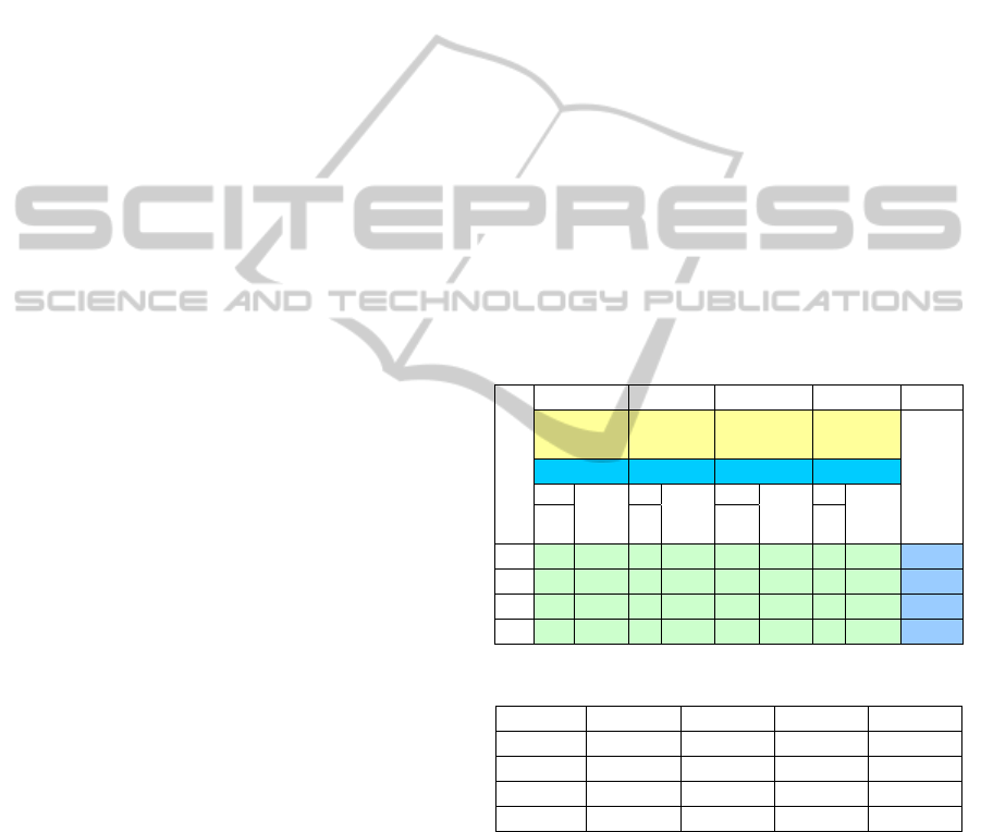
Risk matrix is a widely used qualitative method
for ranking risks (PMI, 2008; Cox, et al, 2005; Cox,
2008). A risk matrix is a table that has several
categories of probability for its rows (or columns)
and several categories of risk impact for its columns
(or rows) respectively. The gray level indicates the
priority of the risks. The deeper gray means higher
risk. The risk level of each region in the risk matrix
should reflect the opinions of stakeholders. Although
people may argue that risk matrix may not rank the
risks accurately (Cox, et al, 2005; Cox, 2008), it can
serve as the basis of quantitative risk analysis. It
provides us the distribution pattern of risks’ priority
at least. Although different projects may use different
risk matrix, the risks with high probability and/or
impact should have high priority. We can use a
typical 5x5 risk matrix to represent this pattern (see
Fig. 1). From Fig. 1, we find that the risk with high
probability or high impact should have a higher
priority than those risks with relatively low
probability and impact. For example, a risk in
(Frequently, Insignificant) region and a risk in
(Seldom, Catastrophic) region should have higher
priority than any risks in the region formed by
(Possible, Unlikely, Seldom) and (Moderate, Minor,
Insignificant).
Frequently
Likely
Possible
Unlikely
Seldom
Probability
Impact
Insignific
ant
Minor Moderate Major Catastrop
hic
Figure 1: A risk matrix.
2.2 Assessment of Risk Impact
One way to assess the risk impact is approximate it
without working out the impacts in different
dimensions, such as time, budget, quality, and scope
(Mcmanus, 2004; Boehm,1991). For example, we
can assess the impacts on a relative scale of (0, 10].
This is commonly used in practice because of its
simplicity. However, this kind of method is
inaccurate.
Very few studies assess the risk impact with due
consideration of the impact of risk in different
dimensions of IT projects. The method proposed by
Ferguson (2004) for assessing risk impact does not
integrate the impact in different dimensions properly.
The basic idea of his method is first divide the risk
impact into 5 levels. Each level associates with a
benchmark and an impact score. The benchmark of
the 5
th
level is established according to the project.
Then, the benchmarks of lower levels are 1/3 of its
immediate upper level. The impact score is
calculated as
Impact score = 3
(l
eve
l
-1
)
(1)
ICEIS 2011 - 13th International Conference on Enterprise Information Systems
26

Each risk can be classified into one impact level
based on practitioners’ judgment and assigned the
impact score of that level. For example, assume a
project, “Project A”, will take 18 months with a
project cost of $3 million, and expect to achieve $1
million revenue in the first year. The benchmark and
the impact score of each level is shown in Table 1.
Then, a risk is assigned an impact score of 9 if it is
classified into level 3.
Table 1: Benchmark and impact score of “Project A”.
Impact
Level
Benchmark
Impact
Score
5
z Overrun by 18 months.
z Overspend by $3M.
z Lose $1M in revenue.
81
4
z Overrun by 6 months.
z Overspend by $1M.
z Lose $333K in revenue.
27
3
z Overrun by 2 months.
z Overspend by 333K.
z Lose $111K in revenue.
9
2
z Overrun by 3 weeks.
z Overspend by $111K.
z Lose $37K in revenue.
3
1
z Overrun by 1 week.
z Overspend by $37K.
z Lose $12K in revenue.
1
This method has two major problems. First, the
granularity is too big to accurately assess the risk
impact. For example, assume that two risks have
impacts in overrun by 4 months and 8 months
respectively. Although they have significant
difference in overrun, they are assigned the same
impact value of 27. Second, it does not consider the
impacts in different impact dimensions. For example,
assume that one risk has impact in overrun by 6
months and overspend by 500K, and the other has
impact in overrun by 6 months and overspend by
100K. Although their overspendings are significantly
different, they may be classified into the same impact
level of 3 according to their major impact in time
dimension and then are assigned the same impact
value of 27.
2.3 Risk Exposure (RE)
RE was introduced by Boehm (1989), and defined as
the multiplication of probability and impact of the
risk.
R
EPI=×
(2)
Although RE is widely used and accepted by
most practitioners, we find that RE can not properly
prioritize the risks. Fig. 2 shows RE contours as a
function of probability and impact, where both
probability and impact range from 0 to 1.
1
Probability
Impact
RE=0.10
RE=0.25
0 1
RE=0.50
Figure 2: Contours of RE.
From Fig. 2, we can find that risks with high
probability and low impact, or high impact and low
probability, have the same RE value as those risks
with relatively low probability and risk. For example,
let’s consider four risks as shown in Table 2. Three
of them, risk
a, b, and c, have the same RE value
0.18. Then, they will have the same priority in risk
response process if we use RE to prioritize risks.
Further, as risk
d has the highest RE value among all
four risks, it has the highest priority. However, risk
a
and
b should have a higher priority than risk c and d,
because the risks with high probability or high
impact should have a higher priority than those risks
with relatively low probability and impact (Boehm,
1989; Mcmanus, 2004; Pandian, 2007). As
demonstrated in this example, we find that RE can
not properly prioritize the risks for certain cases.
Table 2: Four risks and their RE.
Risk Probability Impact RE
a 0.9 0.2 0.18
b 0.2 0.9 0.18
c 0.4 0.45 0.18
d 0.45 0.45 0.20
2.4 Analytic Hierarchy Process (AHP)
Analytic Hierarchy Process (AHP) has been
extensively studied and refined since it was proposed
twenty years ago (Saaty, 1994; Lipovetsky, 1996;
Lipovetsky and Tishler, 1994; Forman and Gass,
2001). It is a structured technique for decision
making. The AHP is most useful when people work
on complex problems which include different stakes
and involve human perceptions and judgment
(Bhushan and Rai, 2004). It calculates a numerical
value, global rating, for alternatives which can be
processed and compared over the entire range of the
problem. The global rating can also be used to
evaluate objects with multiple dimensions (Bhushan
and Rai, 2004; Forman and Gass, 2001). Note that,
although there are many versions of AHP (Bhushan
A NEW METHOD AND METRIC FOR QUANTITATIVE RISK ANALYSIS
27

and Rai, 2004), we will use the standard approach in
this paper for its universality.
The users of AHP need to decompose the
problem into a hierarchy of goal, criteria, sub-criteria
and alternatives first. Then, the weighted-sum
method (WSM) is used for evaluating each
alternative. We can get the weighted rating in each
criterion by multiplying the rating of alternatives in
each criterion and the importance of the criterion.
This product is summed over all the criteria to
generate the global ratings of the alternative.
Mathematically,
1
n
iijj
j
Rating rw
=
=
∑
(3)
where
Rating
i
is the rating of the i
th
alternative, r
ij
is
the rating of the
i
th
alternative in the j
th
criterion, and
w
j
is the weight or importance of the j
th
criterion.
An important issue in using AHP is how to
weight different criteria. One way to do this is
compare all pairs of combinations. The result of the
comparisons can be represented with a square
decision matrix,
A, which is shown in (4). Each
element in the matrix,
a
ij
, represents the relative
importance of the
i
th
criterion compared with the j
th
criterion. The measurement scale used by the AHP is
one of 1 – 9 in absolute numbers. The higher value
means higher comparative importance while 1 means
equal importance. For example, if the
i
th
criterion is
moderately more important than
j
th
criterion, then a
ij
can be assigned 3. On the contrary,
a
ij
can be
assigned 1/3. Based on decision matrix,
A, we can
calculate the weights of different criteria (Saaty,
1994; Bhushan and Rai, 2004).
12 1
12 2
12
1
1/ 1
1/ 1/ 1
n
n
nn
aa
aa
A
aa
⎛⎞
⎜⎟
⎜⎟
=
⎜⎟
⎜⎟
⎝⎠
"
"
#%#
(4)
3 A METHOD TO ASSESS RISK
IMPACT
A risk may have potential impacts on different
dimensions of a project. For example, turnover is a
common risk of many projects. If this risk happens, it
may require some additional schedule time and
additional resource cost to hire and train staff.
Besides that, the quality of product/service may
downgrade since the new team member is not
familiar with the project.
Step 1:
Identify the complete loss for the project in four
risk dimensions: time, budget, quality and scope.
Step 2:
Measure R’s impact in each dimension based on
complete loss of that dimension.
Step 3:
Weight four dimensions and combine the risk
impacts in four dimensions using AHP.
Figure 3: Procedure for assessing risk impact.
A problem of existing methods for risk impact
assessment is they do not combine the impacts in
different dimensions. In order to assess the risk
impact accurately, practitioners can follow our
proposed procedures as shown in Fig. 3.
The first step is identifying what are the complete
loss for a project in its most important four
dimensions, time, budget, quality, and scope (PMI,
2008; Kerzner, 2006). The practitioners should
decide the complete loss in each dimension based on
the constraints and assumptions of the project. As
Jones (1996) reported that “the typical project is 100
percent over budget when it is cancelled”, in many
cases, it is a good choice to set the complete loss of
each dimension to the value that would cause the
project to be cancelled. For example, the complete
loss in the time dimension could be set to 12 months
if the schedule of the project is 12 months.
Practitioners should identify the complete loss
according to specific characteristics of their project.
We use
CL
k
, k=1,…,4, to denote the complete loss in
time, budget, quality, and scope respectively.
The second step is measuring the risk impact in
each dimension based on the complete loss of that
dimension. We use
I
k
, k=1,…,4, to denote the impact
in time, budget, quality, and scope respectively. Then,
the impact of a risk can be represented as a 4-tuple,
(
I
1
, I
2
, I
3
, I
4
). For any risk, we use PL
k
to denote its
potential loss in the
k
th
dimension. Then, the ratio of
PL
k
over CL
k
, can be used to rank the impact in the
k
th
dimension. Note that practitioners should confine
the
PL
k
in the range of [0, CL
k
]. If the estimated PL
k
is bigger than
CL
k
, practitioners can set PL
k
equal to
CL
k
.
k
k
k
PL
I
CL
=
(5)
where,
I
k
ranges in [0, 1]. For example, assume a risk
has a potential loss of 6 months in the time
dimension, and the complete loss in this dimension is
18 months. That is
CL
1
=18 months and PL
1
=6
ICEIS 2011 - 13th International Conference on Enterprise Information Systems
28
months
. Then, the risk impact in the time dimension,
I
1
= PL
1
/ CL
1
=(6 months)/(18 months) = 0.33.
The third step is weighting different impact
dimensions and then calculating the risk impact using
AHP. The practitioners can weight different impact
dimensions based on the characteristics of the project,
enterprise environment factors, past experiences, and
so on. When we use AHP to assess risk impact, the
risks of the project serve as the alternatives in AHP,
the four impact dimensions serve as the criteria in
AHP, and
I
k
serves as the rating in the k
th
criterion.
Then, the risk impact,
I, of a risk is the global rating
of the risk in AHP. If we use
W
k
, k=1,…,4, to denote
the weights of four impact dimensions, time, budget,
quality, and scope respectively, the risk impact,
I, is
calculated with (6) in terms of global rating of AHP.
4
1
kk
k
I
IW
=
=
∑
(6)
where, 0≤
I
k
≤1, 0< W
k
<1 and ∑ W
k
=1.
We next use an example and Table 3 to illustrate
the procedures of assessing risk impact. Assume
there is a project with 12 months schedule and budget
of $200K. The project has 30 quality metrics defined
in requirement and has a size of 100 function points
(FP). We also assume that practitioners found 4 risks
in risk identification. To assess the risk impact of the
risks, the practitioners should define the complete
loss in each dimension based on specific
characteristics of the project first. We assume that the
complete loss in each dimension is overrun by 2
months, overspend by $50K, failed in 5 quality
metrics and missing 30 FP respectively. That is,
CL
1
=2months, CL
2
=$50K, CL
3
=5metrics, CL
4
=30FP.
Second, practitioners should assess the potential loss
of all risks of the project in each dimension. Assume
that the potential losses of those 4 risks in our
example were already assessed by practitioners. Then,
we can compute their impact in each dimension. The
results of this step are shown in the 5
th
row to 8
th
row
of Table 3. Third, practitioners should work out the
decision matrix based on the characteristics of the
project. The decision matrix is shown in Table 4.
This matrix shows that time and quality dimension
have equal importance, both quality and time are
moderately more important than budget and strongly
more important than scope, and budget is moderately
important over scope. Based on the decision matrix,
we can use the method defined in AHP to compute
the weight of each dimension. Practitioners can use
some tools to calculate the weight of each dimension
(For example, an online tool is available at
http://www.isc.senshu-u.ac.jp/~thc0456/EAHP/AHPweb.html.).
The weight of each dimension in this example is
W
1
= 0.379,
W
2
= 0.140, W
3
= 0.400, W
4
= 0.081. After
that, practitioners can calculate the risk impact of
each risk with (6). The results of this step are shown
in the last column of Table 3.
Note that practitioners can use other ways to
measure the complete loss and potential loss in
quality dimension and scope dimension. Our
example assumes that all quality metrics and
functions have the same importance, whereas, in real
project some quality metrics and functions are key
metrics and key functions we can not miss. If a risk
has potential impact on those key metrics and
functions, we should consider the potential loss as a
complete loss.
Note that our method can also be extended to
more dimensions. That is, practitioners can identify
other impact dimensions rather than our proposed
dimensions. To extend our method, practitioners
should identify all impact dimensions first, and then
follow the steps shown in Fig. 3 to assess the risk
impact. The only difference is that practitioners
should consider all identified risk dimensions, not
just our proposed dimensions.
Table 3: Example for assessing risk impact.
Risks
Time Budget Quality Scope
Impact
CL
1
=2mont
hs
CL
2
=$50K CL
3
=5metric
s
CL
4
=30FP
4
1
kk
k
IIW
=
=
∑
W
1
=0.379 W
2
=0.140 W
3
= 0.400 W
4
=0.081
P
L
1
I
1
=
PL
1
/
CL
1
P
L
2
I
2
=
PL
2
/
CL
2
P
L
3
I
3
=
PL
3
/
CL
3
P
L
4
I
4
=
PL
4
/
CL
4
wee
k
K
metri
cs
FP
1
4 0.50 0 0.20 0 0 20 0.67 0.272
2
0 0 0 0.40 3 0.60 10 0.33 0.323
3
2 0.25 0 0.20 2 0.40 5 0.17 0.297
4
0 0 0 0 2 0.40 0 0.33 0.187
Table 4: Decision matrix for the example.
Time Budget Quality Scope
Time 1 3 1 4
Budget 1/3 1 1/3 2
Quality 1 3 1 5
Scope 1/4 1/2 1/5 1
We use AHP to weight different impact
dimensions and combine the impacts of different
dimensions into one single value because of
following reasons. AHP has solid mathematical basis
and “it has been applied literally to hundreds of
examples both real and hypothetical” (Saaty, 2008).
The power and validity of AHP have already been
validated in practices. Compared with the simple
weighted-sum method AHP provides a hierarchy
structure for risk assessment, which is useful when
A NEW METHOD AND METRIC FOR QUANTITATIVE RISK ANALYSIS
29

we want to divide impact dimensions into sub-
dimensions. It also provides us a useful method for
weighting different impact dimensions based on the
decision matrix.
The proposed method for assessing risk impact is
more accurate than other methods, such as
approximate methods and the Ferguson method,
since we not only measure the impacts of different
dimensions but also integrate them together.
4 A NEW METRIC FOR RISK
PRIORITIZATION
4.1 Risk Intensity
As mentioned earlier, RE can not properly address
the priority of the risks. We propose a new metric,
Risk Intensity (RI), to measure the priority of the risk.
We assume that a project includes a set of
n risks
at time
t, RSet(t) = {R
1
, R
2
, …, R
n
}. Both the
probability and the impact of
R
i
, R
i
∈RSet(t), and the
number of risks may change as time elapse. The new
metric, RI, should satisfy following constrains:
1.
∀ R
i
:(P
i
, I
i
), R
j
:(P
j
, I
j
)∈RSet(t), if P
i
= P
j
and
I
i
= I
j
then Pri
i
= Pri
j
;
2.
∀ R
i
:(P
i
, I
i
), R
j
:(P
j
, I
j
)∈RSet(t), if P
i
> P
j
and
I
i
> I
j
then Pri
i
> Pri
j
;
3.
∀ R
i
:(P
i
, I
i
), R
j
:(P
j
, I
j
)∈RSet(t), if P
i
> P
j
and
I
i
= I
j
then Pri
i
> Pri
j
;
4.
∀ R
i
:(P
i
, I
i
), R
j
:(P
j
, I
j
)∈RSet(t), if P
i
= P
j
and
I
i
> I
j
then Pri
i
> Pri
j
;
5.
∀ R
i
:(P
i
, I
i
), R
j
:(P
j
, I
j
)∈ RSet(t), if (P
i
> P
j
and
I
i
< I
j
) or (P
i
< P
j
and I
i
> I
j
), the Pri
i
and
Pri
j
should approximately match the
pattern of the risk matrix in Fig. 1.
where,
Pri
i
and Pri
j
are the priority of risks R
i
and R
j
,
respectively.
A risk can be mapped to a point in the PI
(probability and impact) area (0, 1)×(0 ,1] if we only
focus on risk rather than opportunity. Fig. 4 shows
the mapping of 3 risks and their points in the 2-
dimension PI space. Risks
R
A
:(0.5, 0.5), R
B
:(0.1, 1),
and
R
C
:(0.9, 0.2), are mapped to points A, B, and C
respectively.
impact
1
p
robability
0 1
R
A
:(0.5,0.5)
R
B
:(0.1,1)
RI
B
=1.00
R
E
B
=0.10
C
B
A
RI
C
=0.92
R
E
C
=0.18
R
C
:(0.9,0.2)
RI
A
=0.71
R
E
A
=0.25
Figure 4: RI and RE of risks.
Frequently
Likely
Possible
Unlikely
Seldom
Probability
Impact
Insignific
ant
Minor Moderate Major Catastrop
hic
convex concave
Figure 5: Contours and the risk matrix.
Most practitioners would accept that the risk with
higher probability and higher impact should have
higher priority. Thus, a risk that is further away from
the original point in PI space should have a higher
priority. Based on this idea and the geometric
meaning of Euclidean distance, we define RI as the
Euclidean distance between the risk point and the
original point.
22
R
IPI
=
+ (7)
where,
P and I are the probability and risk impact of
the risk. RI ranges in (0, 1.41). As shown in Fig. 4,
RI of risks
R
A
:(0.5, 0.5), R
B
:(0.1, 1), and R
C
:(0.9, 0.2)
are
RI
A
=0.71, RI
B
=1, and RI
C
=0.92 respectively. It is
easy to verify that RI satisfies constraints 1-4. As
shown in Fig. 6, the contours of RI are convex. Thus,
RI also satisfies constraint 5.
Using the risks shown earlier in Table 2 as
example, the RI and RE of these risks are shown in
Table 5. In this example, we find that RI gives high
priority to those risks which have high probability or
high impact whereas RE does not.
Table 5: Decision matrix for the example.
Risk P I RE RI
a 0.9 0.2 0.18 0.92
b 0.2 0.9 0.18 0.92
c 0.4 0.45 0.18 0.60
d 0.45 0.45 0.20 0.64
ICEIS 2011 - 13th International Conference on Enterprise Information Systems
30
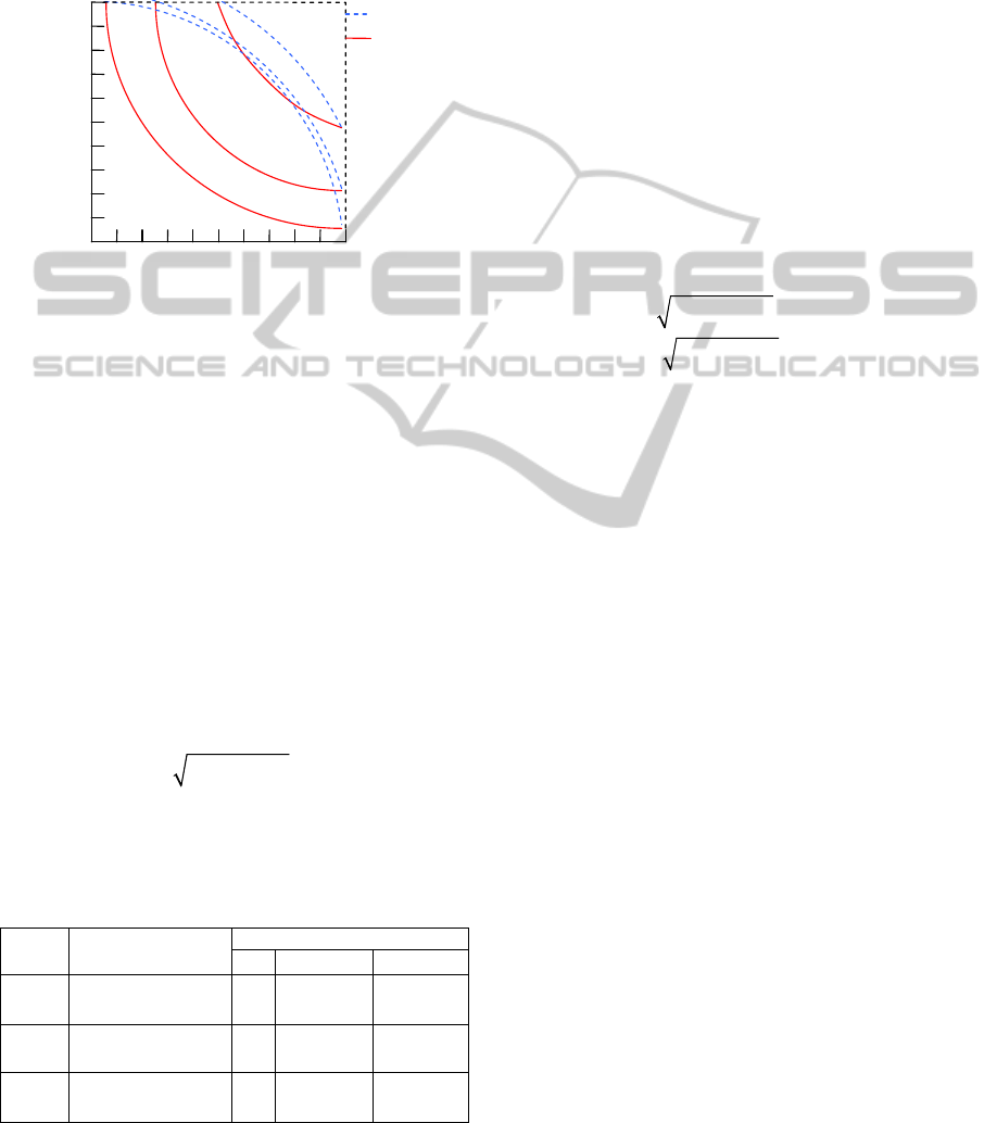
The most important advantage of RI over RE is
that RI matches the risk matrix well while RE not.
Fig. 6 shows contours of RI and RE respectively. It is
easy to find that the RI contours are convex while the
RE contours are concave. RI is more accurate than
RE in risk prioritization when the risk matrix used in
the project shows a convex pattern.
impact
p
robability
1
0 1
RI
RE
RE=0.5
RI =1.12
RE=0.25
RI =1.03
RE=0.10
RI =1.01
Figure 6: Contours of RI and RE.
In risk management, we apply different strategies
for dealing with the risks according to the specific
circumstances of the project. Sometimes, the
practitioners may consider the risk impact slightly
more important than probability. For other cases, the
practitioners may consider the probability slightly
more important than impact. However, both RI in (7)
and RE give equal weight to probability and risk
impact. For example, there are two risks, R
1
:(0.9,
0.2), and R
2
:(0.2, 0.9). If we want to give a higher
weight for risk impact in prioritizing risks (that is, R
2
should be assigned a higher priority than R
1
), both RI
and RE can not distinguish the difference between R
1
and R
2
.
To solve this problem, we can weight probability
and risk impact differently, and (7) can be improved
as (8).
22
()
R
IPwI+⋅=
(8)
where,
w is a positive real number and is used to
weight probability and risk impact. Table 6 shows
the functions of
w.
Table 6: Functions of variable w in (8).
w
Function
Exam
p
le
w R
1
:(0.9, 0.2) R
2
:(0.2, 0.9)
w>1 I is more important
than P
1.05 RI
1
=0.924 RI
2
=0.966
w=1 Both P and I have
the same weight
1.00 RI =0.922 RI
2
=0.922
0<w<1 P is more important
than I
0.95 RI
1
=0.920 RI
2
=0.878
From Table 6, we can find that w can be used to
weight probability and risk impact differently. In
practice, an easy way can be used to determine the
value of
w. Practitioners first assume the weight of
probability,
w
p
is 1, and then decide the comparative
weight of risk impact,
w
I
, according to the
circumstances of the project, and
w can be derived
from
w
I
/w
p
.
It’s easy to verify that (8) satisfies constraints 1-4.
Since the introduction of
w only change the range of
I from (0, 1] to (0, w], and does not change the
contours of RI from convex to concave, (8) also
satisfies constraint 5.
According to above analysis, RI not only can
match the risk matrix shown in Fig. 1 well but also
can weight probability and risk impact differently,
whereas RE can not.
To include risk events that offer opportunity, the
definition of RI is enhanced as (9).
22
22
() 0
() 0
PwIifI
RI
PwIifI
+
⋅>
=
−
+⋅ <
⎧
⎪
⎨
⎪
⎩
(9)
4.2 A Case Study
To evaluate RI, we conduct an empirical study on
applying it to a real project. Project A is a project
which enhanced System X to allow customers to
submit documents and related information
electronically via Internet.
The practitioners identified 25 risks after the
project planning and system design phase. Table 7
shows these risks and their probability, impact and
risk level. Both the probability and impact of the risk
are ranked from 0 to 5 (and can be normalized from 0
to 1 as shown in bracket), where a higher probability
value represents a higher chance of occurrence and a
higher impact value represents a higher negative
effect. According to the risk matrix used by the
organization (see Fig. 7), each risk was classified as
Low Risk (L), Medium Low Risk (M-), Medium
Risk (M), Medium High Risk (M+), or High Risk
(H).
In risk prioritization, those risks with the same
probability and impact have the same priority. For
example, Risk 7, 19, 23 and 24 have the same
priority. Thus, we focus on those risks with different
probability and/or impact (Risk 1, 2, 3, 5, 7, 8, 10, 11
and 22) in the following prioritization exercise.
In this project, the practitioners use two rules to
prioritize the risks.
A NEW METHOD AND METRIC FOR QUANTITATIVE RISK ANALYSIS
31

Table 7: Functions of variable w in (8).
Risk No. 1 2 3 4 5 6 7
Probabil
ity
2
(0.4)
3
(0.6)
1
(0.2)
3
(0.6)
1
(0.2)
1
(0.2)
2
(0.4)
Impact
4
(0.8)
4
(0.8)
3
(0.6)
4
(0.8)
4
(0.8)
3
(0.6)
3
(0.6)
Level M+ H M- H M M- M
Risk No. 8 9 10 11 12 13 14
Probabil
ity
3
(0.6)
2
(0.4)
4
(0.8)
4
(0.8)
4
(0.8)
4
(0.8)
3
(0.6)
Impact
3
(0.6)
4
(0.8)
4
(0.8)
3
(0.6)
3
(0.6)
4
(0.8)
3
(0.6)
Level M+ M+ H H H H M+
Risk No. 15 16 17 18 19 20 21
Probabil
ity
3
(0.6)
2
(0.4)
4
(0.8)
3
(0.6)
2
(0.4)
4
(0.8)
3
(0.6)
Impact
3
(0.6)
4
(0.8)
3
(0.6)
4
(0.8)
3
(0.6)
4
(0.8)
3
(0.6)
Level M+ M+ H H M H M+
Risk No. 22 23 24 25
Probabil
ity
2
(0.4)
2
(0.4)
2
(0.4)
3
(0.6)
Impact
2
(0.4)
3
(0.6)
3
(0.6)
4
(0.8)
Level M- M M H
0 1 2
3 4
Im
p
act
5
1
2
3
4
M M+ H H
M- M M+ H
L M- M M+
L L M- M
Probability
5
Figure 7: Risk matrix used by the organization.
First, the risk with higher risk level has higher
priority. Second, for any two risks, R
a
and R
b
, in the
same risk level, if (P
a
>P
b
and I
a
>I
b
), or (P
a
>P
b
and
I
a
=I
b
), or (P
a
=P
b
and I
a
>I
b
) then R
a
has higher priority
than R
b
, otherwise the risk with higher impact value
has higher priority as the practitioners pointed out
that “impact is usually easier to be estimated than
probability and people trend to put more efforts on
those higher impact risks”. We prioritize Risk 1, 2, 3,
5, 7, 8, 10, 11 and 22 according to these two rules.
The results are shown in column 5 of Table 8 and this
prioritized list can serve as “standard list” in the
evaluation of RI. Note that the lower priority value
indicates higher priority.
We also compute RE, RI and RI (
w=1.05) with
normalized probability and impact value and
prioritize the risks respectively. The RE, RI and RI
(w=1.05) values of the risks and the priority values
which derived from RE, RI and RI (
w=1.05)
respectively are shown in column 6-8 of Table 8.
Note that priority values are shown in bracket.
In this project, we can find that RE has more
conflicts with the “standard list” than RI. From Table
8, it is easy to find that RI better match the “standard
list” than RE, and RI (
w=1.05) better match the
“standard list” than RI. First, the RE does not
correctly prioritize the risks in different risk levels for
certain cases whereas RI does. For example, Risk 22
with M- risk level should have lower priority than
Risk 5. RE wrongly give them the same priority,
however RI and RI (
w=1.05) prioritize them correctly.
Second, for the risks in the same risk level, RE does
not correctly prioritize them in some cases. For
example, Risk 1 should have higher priority than
Risk 8, and Risk 5 should also has higher priority
than Risk 7. RE wrongly prioritize them, but RI and
RI (
w=1.05) could prioritize them correctly. Further,
in this project, the practitioners view the impact more
important than the probability. Then the RI with w>1
could satisfy the need of the practitioners to a greater
degree. We can find that RI (
w=1.05) could
distinguish Risk 2 and Risk 11, whereas both RE and
RI can not. According to above discussion, we can
draw a conclusion that, in this project, RI is better
than RE in risk prioritization.
Table 8: Priority, RE and RI of 9 risks.
Risk
No.
P I Level Priority RE RI
RI
(w=1.05)
10 4
(0.8)
4
(0.8)
H 1
0.64
(1)
1.13
(1)
1.16
(1)
2 3
(0.6)
4
(0.8)
H 2
0.48
(2)
1
(2)
1.03
(2)
11 4
(0.8)
3
(0.6)
H 3
0.48
(2)
1
(2)
1.02
(3)
1 2
(0.4)
4
(0.8)
M+ 4
0.32
(5)
0.89
(4)
0.93
(4)
8 3
(0.6)
3
(0.6)
M+ 5
0.36
(4)
0.85
(5)
0.87
(5)
5 1
(0.2)
4
(0.8)
M 6
0.16
(7)
0.82
(6)
0.86
(6)
7 2
(0.4)
3
(0.6)
M 7
0.24
(6)
0.72
(7)
0.75
(7)
3 1
(0.2)
3
(0.6)
M- 8
0.12
(9)
0.63
(8)
0.66
(8)
22 2
(0.4)
2
(0.4)
M- 9
0.16
(7)
0.57
(9)
0.58
(9)
Note that RI is not always better than RE. For
example, if there is a Risk26:(4, 1) in the project. It
should have lower priority than Risk5 and Risk7, that
ICEIS 2011 - 13th International Conference on Enterprise Information Systems
32

is, Risk5> Risk7> Risk26. RE prioritize them as
Risk7> Risk5= Risk26, RI prioritize them as Risk5=
Risk26> Risk7, and RI (
w=1.05) prioritize them as
Risk5> Risk26> Risk7. In this case, none of the
metrics can prioritize the risks correctly.
5 CONCLUSIONS
In this paper, we identified the research gap in
measuring risk impact and some problems with the
common indicator RE for prioritizing risks. To
bridge this gap, we propose a method for measuring
risk impact by using AHP. Then, we propose risk
intensity (RI) to prioritize the risks of a project.
According to our analysis in section III and IV, our
method for assessing risk impact would be more
accurate than other existing methods and RI is better
than RE in prioritizing risks.
Our study has some limitations. First, although the
proposed method for assessing risk impact would be
more accurate than other methods according to our
analysis, it has not been fully evaluated in practice.
Second, we only evaluate RI in one project. The
usefulness of RI needs to be confirmed by applying it
to more projects in the future. We plan to evaluate
the validity of our method for assessing risk impact
and the practical usage of RI with more real-life
projects in the near future.
REFERENCES
Bhushan, N. and Rai, K., 2004. Strategic Decision Making:
Applying the Analytic Hierarchy Process. London,
Springer.
Boehm, B., 1989. Software Risk management, IEEE
Computer Society Press.
Boehm, B., 1991. “Software risk management: principles
and practices”, IEEE software, Vol.8, No.1, pp.32-41.
Cox, L. A., et al, 2005. Huber, “Some limitations of
qualitative risk rating systems”, Risk Analysis, Vol.25
No.3, pp.651-662.
Cox, L. A. 2008, “What's Wrong with Risk Matrices?”,
Risk Analysis, Vol.28, No.2, pp.497-512.
Ferguson, R. W., 2004, “A project risk metric”, CrossTalk:
The Journal of Defense Software Engineering, Vol.17,
No.4, pp.12-15.
Forman, E. H., and Gass, S. I., 2001. "The analytical
hierarchy process-an exposition", Operations
Research, Vol.49, No.4, pp.469-486.
Gluch, D. P., 1994. “A Construct for Describing Software
Development Risks”, SEI Technical Report
CMU/SEI-94-TR-14, SEI, Pittsburgh, PA.
Jones, C., 1996. Patterns of Software Failure and Success,
Boston, MA: International Thompson Computer Press.
Kähkönen, K., 2001. “Integration of Risk and Opportunity
Thinking in Projects”, Presented in Proceedings of 4
th
European Project management Conference, London,
Jun, PMI Europe 2001.
Kerzner, H., 2006. Project management: a systems
approach to planning, scheduling, and controlling, 9
th
edition, Hoboken, N.J.
Lipovetsky, S. and Tishler, A., 1994. “Linear methods in
multimode data analysis for decision making”,
Computers and Operations Research, Vol.21, No.2,
pp.169-183.
Lipovetsky, S., 1996. “The synthetic hierarchy method: an
optimizing approach to obtaining priorities in the
AHP”, European Journal of Operational Research, 93,
pp.550-569.
Mcmanus, J., 2004. Risk management in Software
Development Projects, Elsevier, Burlington, MA.
Pandian, C. R., 2007. Applied software risk management:
a guide for software project managers, Auerbach,
Boca Raton, Fla.
PMI, 2008. A guide to the project management body of
knowledge, 4
th
edition, Project management Institute,
Newtown, PA.
Saaty, T. L., 1994. Fundamentals of Decision Making and
Priority Theory with Analytic Hierarchy Process.
Pittsburgh, RWS.
Saaty, T. L., 2008. "Relative Measurement and its
Generalization in Decision Making: Why Pairwise
Comparisons are Central in Mathematics for the
Measurement of Intangible Factors - The Analytic
Hierarchy/Network Process", RACSAM, Vol.102, No.2,
pp.251-318.
Sherer, S., 2004. “Managing risk beyond the control of IS
managers: the role of business management”,
Proceedings of 37
th
Hawaii International Conference
on System Sciences, Hawaii, Track 8.
White, B. E., 2006. “Enterprise Opportunity and Risk”,
INCOSE 2006 Symposium Proceedings, Orlando.
A NEW METHOD AND METRIC FOR QUANTITATIVE RISK ANALYSIS
33
