ON THE DISTRIBUTION OF SOURCE CODE FILE SIZES

Israel Herraiz

Technical University of Madrid, Madrid, Spain

Daniel M. German

University of Victoria, Victoria, Canada

Ahmed E. Hassan

Queen’s University, Kingston, Canada

Keywords:

Mining software repositories, Software size estimation, Open source.

Abstract:

Source code size is an estimator of software effort. Size is also often used to calibrate models and equations

to estimate the cost of software. The distribution of source code ﬁle sizes has been shown in the literature to

be a lognormal distribution. In this paper, we measure the size of a large collection of software (the Debian

GNU/Linux distribution version 5.0.2), and we ﬁnd that the statistical distribution of its source code ﬁle sizes

follows a double Pareto distribution. This means that large ﬁles are to be found more often than predicted by

the lognormal distribution, therefore the previously proposed models underestimate the cost of software.

1 INTRODUCTION

Source code size is a simple, yet powerful metric

for software maintenance and management. Over the

years, much research has been devoted to the quest

for metrics that could help optimize the allocation

of resources in software projects, both at the devel-

opment and maintenance stages. Two examples of

these are McCabe’s cyclomatic complexity (McCabe,

1976) and Halstead’s software science metrics (Hal-

stead, 1977). In spite of all the theoretical consider-

ations that back up these metrics, previous research

shows that simple size metrics are highly correlated

with them (Herraiz et al., 2007), or that these met-

rics are not better defect predictors than just lines of

code (Graves et al., 2000).

Perhaps due to these facts, software size, rather

than many other more sophisticated metrics, has been

used for effort estimation. Standard models like

COCOMO are now widely used in industry to esti-

mate the effort needed to develop a particular piece of

software, or to determine the number of billable hours

when building software (Boehm, 1981).

In recent years, besides the previously mentioned

works, the statistical properties of software size have

attracted some attention in research. Recent research

shows that the statistical distribution of source code

ﬁle sizes is a lognormal distribution (Concas et al.,

2007), and some software size estimation techniques

built on that ﬁnding (Zhang et al., 2009). Some other

preliminary research conﬂicts with this ﬁnding for

the distribution of size, proposing that the statistical

distribution of source code ﬁle sizes follows a dou-

ble Pareto distribution (Herraiz et al., 2007; Herraiz,

2009).

All the mentioned works use publicly available

software, so they can be repeated and veriﬁed by third

parties. These are crucial aspects to determine with-

out further doubt which is the statistical distribution

of size. However, some of these studies (Zhang et al.,

2009; Concas et al., 2007) are based on a few case

studies, with the consequent risk of lack of generality,

opening the door to possible future conﬂicting stud-

ies. To overcome these drawbacks, we report here the

results for a very large number of software projects,

which source code have been obtained from the De-

bian GNU/Linux distribution, release 5.0.2. Our sam-

ple contains nearly one million and a half ﬁles, ob-

tained from more than 11, 000 source packages.

The main contributions of this paper are :

Herraiz I., German D. and Hassan A..

ON THE DISTRIBUTION OF SOURCE CODE FILE SIZES.

DOI: 10.5220/0003426200050014

In Proceedings of the 6th International Conference on Software and Database Technologies (ICSOFT-2011), pages 5-14

ISBN: 978-989-8425-77-5

 2011 SCITEPRESS (Science and Technology Publications, Lda.)

• Software size’s distribution is a double Pareto

This implies that the distribution of software size

is a particular case of the distribution of the size

of ﬁlesystems (Mitzenmacher, 2004b), and it also

conﬁrms previous results based on other case

studies (Herraiz et al., 2007; Herraiz, 2009).

• Estimation techniques based on the lognormal

distribution underestimate the potential size of

software

And therefore they underestimate its cost. We cal-

culate the bias of lognormal models compared to

the size estimated using a double Pareto model.

The rest of the paper is organized as follows. Sec-

tion 2 gives an overview of the related work. Sec-

tion 3 describes the data sources and the methodol-

ogy used in our study. Section 4 shows our approach

to determine the shape of the statistical distribution

of software size. Section 5 compares the lognormal

and double Pareto distributions for software estima-

tion, also showing how the lognormal distribution al-

ways underestimates the size of large ﬁles. For clar-

ity purposes, all the results are brieﬂy summarized in

section 6. Section 7 discusses some possible threats

to the validity of our results. Section 8 discusses some

possible lines of further work. And ﬁnally, section 9

concludes this paper.

2 RELATED WORK

In the mathematics and computer science communi-

ties, the distribution of ﬁle sizes has been an object

of intense debate (Mitzenmacher, 2004a). Some re-

searchers claim that this distribution is a lognormal,

and some others claim that it is a power law. In some

cases, lognormal distributions ﬁt better some empir-

ical data, and in some other cases power law distri-

butions ﬁt better. However, the generative processes

that give birth to those distributions, and the possible

models that can be derived based on those processes,

are fundamentally different (Mitzenmacher, 2004b).

Power-laws research was already a popular topic

in the software research community. Clark and

Green (Clark and Green, 1977) found that the point-

ers to atoms in Lisp programs followed the Zipf’s law,

a form of power law. More recent studies have found

power laws in some properties of Java programs, al-

though other properties (some of them related to size)

do not have a power law distribution (Baxter et al.,

2006). But it is only in the most recent years when

some authors have started to report that this distri-

bution might be lognormal, starting the old debate

previously found for ﬁle sizes in general. Concas et

al. (Concas et al., 2007) studied an object-oriented

system written in Smalltalk, ﬁnding evidences of both

power law and lognormal distributions in its proper-

ties. Zhang et al. (Zhang et al., 2009) conﬁrmed some

of those ﬁndings, and they proposed that software size

distribution is lognormal. They also derive some es-

timation techniques based on that ﬁnding, aimed to

determine the size of software. Louridas et al. (Louri-

das et al., 2008) pointed out that power laws might

not be the only distribution found in the properties of

software systems.

For the more general case of sizes of ﬁles of any

type, Mitzenmacher proposed that the distribution is

a double Pareto (Mitzenmacher, 2004b). This result

reconciles the two sides of the debate. But more inter-

estingly, the generative process of double Pareto dis-

tributions mimics the actual work-ﬂow and life cycle

of ﬁles. He also shows a model for the case of ﬁle

sizes, and some simulation results. The same distribu-

tion was found in the case of software (Herraiz et al.,

2007; Herraiz, 2009), for a large sample of software,

although the results were only for the C programming

language.

The Debian GNU/Linux distribution has been the

object of research in previous studies (Robles et al.,

2005; Robles et al., 2009). It is one of the largest

distributions of free and open source software.

In the spirit of the pioneering study by Knuth in

1971 (Knuth, 1971), where he used a survey approach

of FORTRAN programs to determine the most com-

mon case for compiler optimizations, we use the De-

bian GNU/Linux distribution with the goal of enlight-

ening this debate about the distribution of software

size, extending previous research to a large amount of

software, written in several programming languages,

and coming from a broad set of application domains.

3 DATA SOURCE AND

METHODOLOGY

We retrieved the source code of all the source pack-

ages of the release 5.0.2 of the Debian GNU/Linux

distribution. We used both the main and contrib sec-

tions of distribution, for a total of 11, 571 source code

packages, written in 30 different programming lan-

guages, with a total size of more than 313 MSLOC,

and more than 1, 300, 000 ﬁles. Figure 1 shows the

relative importance of the top seven programming

languages in this collection; they account more than

90% of the ﬁles.

We measured every ﬁle in Debian, using the

SLOCCount tool by David A. Wheeler

. This tool

Available at http://www.dwheeler.com/sloccount

ICSOFT 2011 - 6th International Conference on Software and Data Technologies

C C++ Shell Java Python Perl Lisp

% SLOC

0 10 20 30 40

Figure 1: Top seven programming languages in Debian

(representing 90% of Debian’s size). The vertical axis

shows the percentage of the overall size.

measures the size of ﬁles in SLOC, which is number

of source code lines, excluding blanks and comments.

Table 1 shows a summary of the statistical proper-

ties of this sample of ﬁles, for the overall sample and

for the top seven programming languages. Approxi-

mately half of Debian is written in C, and almost three

quarters of it is written in either C or C++. The large

number of shell scripts is mainly due to scripts used

for build, and installation purposes; shell scripting is

present in about half of the packages in Debian.

We divided the collection of ﬁles into 30 groups,

one for each programming language and another one

for the overall sample, and estimated the shape of the

statistical distribution of size. For this estimation, we

plotted the Complementary Cumulative Distribution

Function (CCDF) for the top seven programming lan-

guages. The Cumulative Distribution Function (CDF)

is the integral of the density function, and its range

goes from zero to one. The CCDF is the complemen-

tary of the CDF. All these three functions (density

function, CDF and CCDF) show the same informa-

tion, although their properties are different. For in-

stance, in logarithmic scale, a power law distribution

appears as a straight line in a CCDF, while a lognor-

mal appears as a curve. So the CCDF can be used

to distinguish between power laws and other kind of

distributions.

In a CCDF, the double Pareto distribution appears

as a curve with two straight segments, one at the low

values side, and another one at the high values side.

The difference between a lognormal and a power law

at very low values is negligible, and therefore imper-

ceptible in a plot. This means that in a CCDF plot

the main difference between a lognormal and a dou-

ble Pareto is only spotted at high values. In any case,

for our purposes, it is more important to focus on the

high values side. A difference for very small ﬁles

(e.g. < 10 SLOC) is harmless. However, a difference

for large ﬁles (e.g. > 1000 SLOC) may have a great

impact in the estimations.

To estimate the shape of the distribution, we use

the method proposed by Clauset et al. (Clauset et al.,

2007); in particular, as implemented in the GNU

R statistical software (R Development Core Team,

2009). They argue that power law data are often ﬁt-

ted using standard techniques like least squares re-

gression, that are very sensible to observations cor-

responding to very high values. For instance, a new

observation at a very high value may greatly shift the

scaling factor of a power law. The result is that the

level of conﬁdence for the parameters of the distribu-

tion obtained using those methods is very low.

Clauset et al. propose a different technique, based

on maximum-likelihood, that allows for a goodness-

of-ﬁt test of the results. Furthermore, their technique

can deal with data that deviate from the power law

behavior for values lower than a certain threshold,

providing the minimum value of the empirical data

that belongs to a power law distribution. For double

Pareto distributions, that value can be used to calcu-

late the point where the data changes from lognormal

to power law. That shifting value can be used to de-

termine at what point the lognormal estimation model

starts to deviate from the actual data, and to quantify

the amount of that deviation.

4 DETERMINING THE SHAPE

OF THE SIZE DISTRIBUTION

As Table 1 shows, evidenced by the difference be-

tween the median and the average values, our data is

highly right skewed. This is typical of lognormal or

power law-like distributions. There exist many differ-

ent methods to empirically determine the distribution

of a data set. Here we use a combination of different

statistical techniques, to show that in our case, that

the studied size distribution is a double Pareto one.

We ﬁrst show some results for the global sample, and

later we will split our results by programming lan-

guage.

Histograms are a simple tool that can help to ﬁnd

the distribution behind some data. When the width of

the bars is decreased till nearly zero, we have a den-

sity function, that is a curve that resembles the shape

of the histogram. Although a density function is only

deﬁned for continuous data, we can estimate it for our

discrete data, and use it to determine the shape of the

distribution. For the case of our sample, that function

is shown in Figure 2. Note that the horizontal axis

shows SLOC using a logarithmic scale.

Because our data are integers values and discrete,

the estimation of the density function tries to inter-

polate the missing values, showing some “jumps” for

ON THE DISTRIBUTION OF SOURCE CODE FILE SIZES

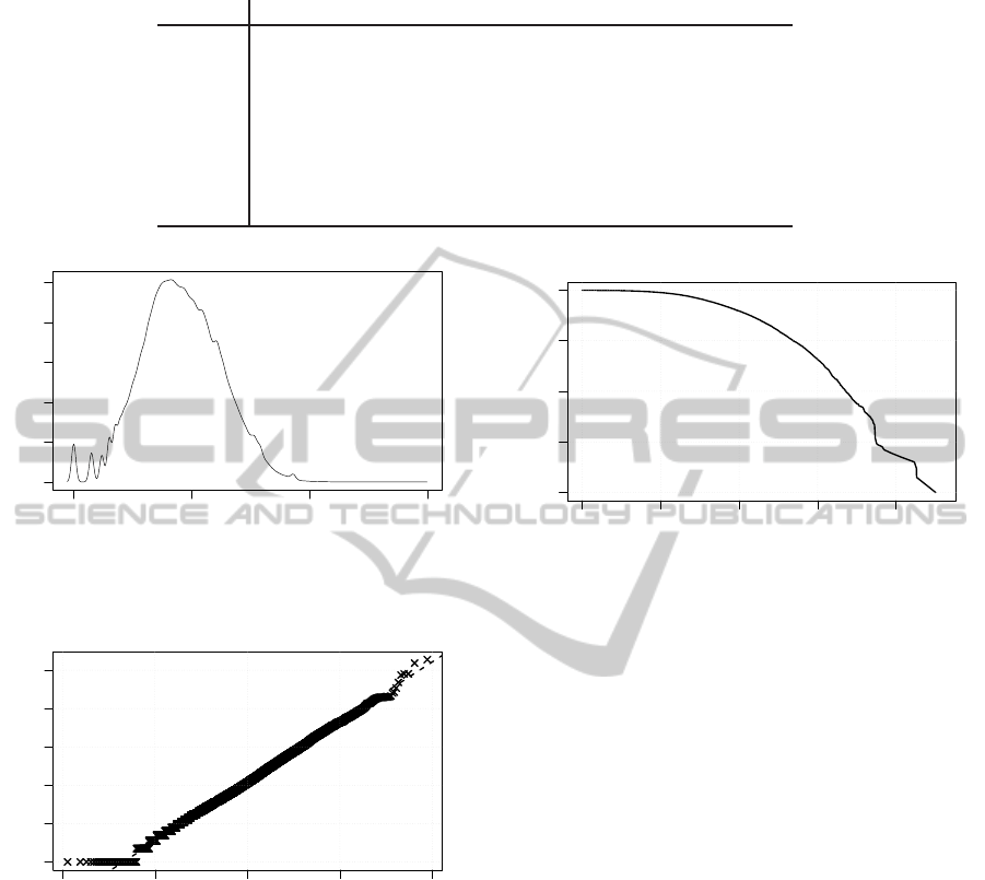
Table 1: Properties of the sample of ﬁles. Values in SLOC.

Lang Num. of ﬁles Max. Avg. Median Total

Overall 1, 355, 752 765, 108 231 63 313, 774, 217

C 498, 484 765, 108 306 85 152, 368, 424

C++ 332, 652 172, 487 193 58 64, 267, 501

Shell 66, 107 46, 497 409 62 27, 038, 314

Java 158, 414 28, 784 109 43 17, 334, 539

Python 63, 590 65, 538 156 59 9, 888, 159

Perl 48, 055 58, 164 188 69 9, 037, 066

Lisp 21, 101 105, 390 373 132 7, 870, 134

1e+00 1e+02 1e+04 1e+06

0.00 0.10 0.20

SLOC

Density

Figure 2: Density probability function for the overall sam-

ple. Horizontal axis shows SLOC in logarithmic scale.

−4 −2 0 2 4

0 2 4 6 8 10

Theoretical Quantiles

Sample Quantiles

Figure 3: Quantile-quantile plot of the overall sample. Log-

arithmic scale.

very low values. The most important feature is that

it shows that the logarithm of size is symmetric, and

that the shape of the curve somehow resembles a

bell-shaped normal distribution, meaning that the data

could belong to a lognormal distribution.

To determine whether the data is lognormal or not,

we can compare its quantiles against the quantiles of

a theoretical reference normal distribution. Such a

comparison is done using a quantile-quantile plot. An

example of such a plot is shown in Figure 3,

In that plot, if the points fall over a straight line,

they belong to a lognormal distribution. If they do

1 10 100 1000 10000

1e−04 1e−02 1e+00

SLOC

CCDF

Figure 4: Complementary cumulative distribution function

of the overall sample.

not, then the distribution must be of another kind. The

shape shown in Figure 3 is similar to the proﬁle of a

double Pareto distribution. The main body of the data

is lognormal, and so it appears as a straight line in the

plot (the points fall over the dashed line that is shown

as a reference). Very low and very high values deviate

from linearity though. However, with only that plot,

we cannot say whether the tails are power law or any

other distribution.

Power laws appear as straight lines in a

logarithmic-scale plot of the cumulative distribution

function (or its complementary). Therefore, combin-

ing the previous plots with this new plot, we can fully

characterize the shape of the distribution. Figure 4

shows the logarithmic-scale plot of the complemen-

tary cumulative distribution function for the overall

sample. The main lognormal body clearly appears

as a curve in the plot. The low values hypothetical

power law cannot be observed, because at very low

values the difference between a power law and a log-

normal is negligible. The high values power law does

not clearly appear either. It seems that the high values

segment is straight, but at a ﬁrst glance it cannot be

distinguished from other shapes.

Using the methodology proposed by Clauset et

al. (Clauset et al., 2007), we estimate the parame-

ters of the power law distribution that better ﬁt the

ICSOFT 2011 - 6th International Conference on Software and Data Technologies

Table 2: Parameters of the power law tails for the top seven

programming languages and the overall sample.

Lang. α x

min

D p

Overall 2.73 1, 072 0.01770 0.1726

C 2.87 1, 820 0.01694 0.5349

C++ 2.80 1, 258 0.01202 0.5837

Shell 1.71 133 0.13721 ∼ 10

−14

Java 3.17 846 0.01132 0.6260

Python 2.90 826 0.01752 0.2675

Perl 2.23 137 0.02750 ∼ 10

−5

Lisp 2.73 1, 270 0.01996 0.5229

tail of our data, and calculate the Kolmogorov dis-

tance, a measure of the goodness of ﬁt. We can also

calculate the transition point at which the data stops

being power law. In the following, we will refer to

that point as the threshold value. With that threshold

value, we can separate the data in at least two different

regions: data which follows a lognormal distribution

and data which follows a power law distribution. The

values estimated for the top seven programming lan-

guages are shown in Table 2. It also includes the p

values resulting from the hypothesis testing, using the

Kolmogorov-Smirnov test.

The second column is the scaling parameter of

the power law. The third column is the threshold

value: ﬁles with sizes higher than that value belong

to the power law side of the double Pareto distribu-

tion. The fourth column is the Kolmogorov distance.

It is the maximum difference between the empirical

CCDF and the CCDF of the power law with the es-

timated parameters. Lower values indicate better ﬁts.

But those values must be tested to determine whether

they are too high to reject the power law hypothesis.

The result of the hypothesis testing is shown in the

ﬁfth column. In this case, the null hypothesis is that

the Kolmogorov distance is null, and the alternate hy-

pothesis is that the Kolmogorov distance is not null.

A null Kolmogorov distance implies that the distribu-

tion of the data is a power law. For a 99.99% sig-

niﬁcance level (p = 0.01), all the programming lan-

guages except shell and Perl are ﬁtted by a power law

(for sizes over the threshold shown in the third col-

umn, of course).

In short, for the case of shell and Perl ﬁles, the

high values tail is not a power law. For the rest of pro-

gramming languages, the high values tail is a power

law.

Regarding the parameters of the lognormal dis-

tribution, we use the standard maximum-likelihood

estimation routines included in the R statistical

package. In this case, the ﬁtting procedure is more

straightforward, as we have already shown with the

quantile-quantile plot (Figure 3) that the data is very

Table 3: Parameters of the lognormal body for the top seven

programming languages and the overall sample.

Lang. ¯x s

D p

Overall 4.1262 1.4857 0.0436 0.0444

C 4.3421 1.5651 0.0448 0.0365

C++ 4.1182 1.2598 0.0363 0.1447

Shell 2.8480 1.3118 0.0656 0.0005

Java 3.7477 1.2627 0.0411 0.0697

Python 3.9543 1.3972 0.0416 0.0340

Perl 3.5272 0.9533 0.0700 ∼ 10

−16

Lisp 4.6485 1.3834 0.0381 0.1265

close to a lognormal, except for the tails. Table 3

shows the parameters of the lognormal distribution,

the Kolmogorov distance, and the results of the

hypothesis testing for the lognormal ﬁtting. Again,

with a signiﬁcance level of 99.99% (p = 0.01), for

small ﬁles, the size distribution of the programming

languages is lognormal—except for shell and Perl.

The distribution of size for all the program-

ming languages is a double Pareto, except for

the case of the shell and Perl programming

languages. This means that ﬁles can be di-

vided in two groups: small and large. The

frontier value between these two regions is

the threshold, x

min

, shown in Table 2.

5 SIZE ESTIMATION USING THE

LOGNORMAL AND DOUBLE

PARETO DISTRIBUTIONS

Software size can be estimated using the shape of the

distribution of source code ﬁle sizes, and knowing the

number of ﬁles that are going to be part of the sys-

tem. Size estimation can also be used for software

effort estimation. Analytical formulas for the case of

Java have even been proposed in the literature (Zhang

et al., 2009). Those formulas are based on the fact

that program size distribution is a lognormal, and use

the CCDF for the estimations.

For small ﬁles, the difference between a log-

normal or a double Pareto distribution is negligible.

However, for large ﬁles, this difference may be high.

This means that the proposed estimation models and

formulas can be very biased for large ﬁles.

Figure 5 compares the CCDF of the ﬁles written

in Lisp, with the double Pareto and lognormal esti-

mations of the CCDF. The threshold value is shown

with a vertical dashed line. For values higher than

the threshold, the lognormal model underestimates

ON THE DISTRIBUTION OF SOURCE CODE FILE SIZES

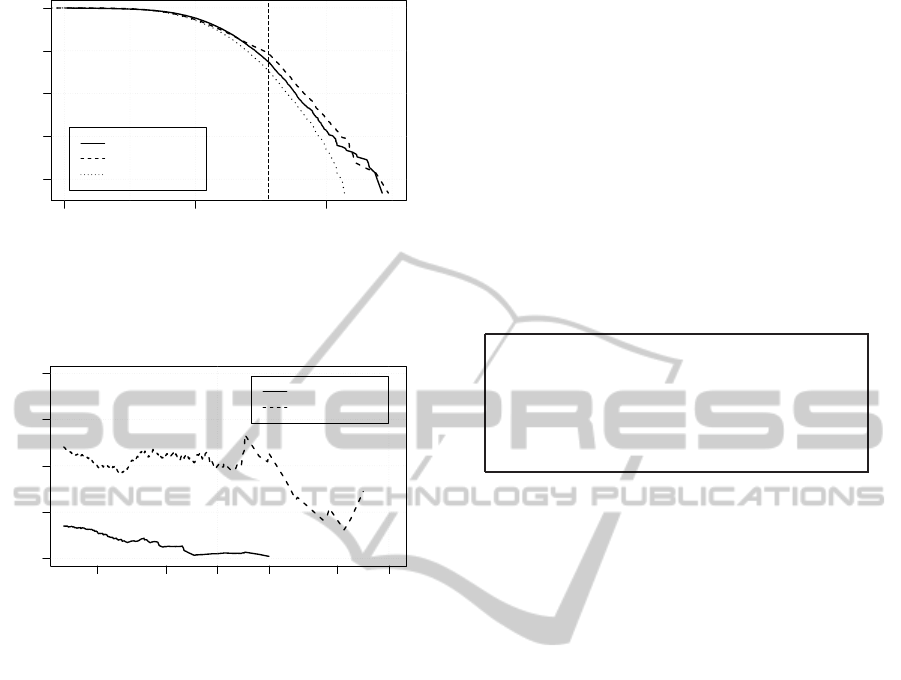
1 100 10000

1e−04 1e−02 1e+00

SLOC

P[X > x]

Data

Double Pareto

Lognormal

Figure 5: CCDF for the Lisp language, comparing the dou-

ble Pareto and lognormal models. Threshold value shown

as a vertical dashed line.

2e+03 5e+03 1e+04 2e+04 5e+04 1e+05

−100 −50 0 50 100

SLOC

Lognormal

Double Pareto

Figure 6: Relative error in percentage for the CCDF of the

lognormal and double Pareto models, compared against the

CCDF of the sample. Only for ﬁles written in Lisp.

the size of the system, and this bias grows with the

size of ﬁle size – the bigger the ﬁle the more the bias.

Figure 6 shows the relative error of the lognormal

and double Pareto models, for the case of the Lisp

language, when predicting the size of large ﬁles. The

CCDF of the ﬁtted models were compared against the

CCDF of the actual sizes of the ﬁles. The lognormal

model always underestimates the size of ﬁles (nega-

tive relative error). The difference for large ﬁles is

so large that it cannot even be calculated because of

overﬂow errors.

The same pattern appears for the rest of program-

ming languages, as shown in Figure 7. The lognormal

model has a permanent bias that underestimate the

size of large. The reason is that ﬁles above a certain

threshold do not belong to that kind of distribution,

but to the power law tail of a double Pareto distribu-

tion.

Although large ﬁles are not as numerous (see

Figure 8), their contribution to the overall size is

as important as small ﬁles’ contribution. Figure 9

shows the relative importance of small and large

ﬁles for all the programming languages that have

been identiﬁed as double Pareto. The bottom part

(dark) of every column is the contribution of small

ﬁles, and the top part (clear) the contribution by

large ﬁles. Small ﬁles are those ﬁles with a size

lower than the threshold value shown in Table 2.

We do not include the Shell and Perl languages

because the distribution is not a double Pareto, and

therefore the threshold values do not make sense in

those cases. The plot clearly shows that the relative

contribution of large ﬁles is quite notable, even if

large ﬁles are only a minority. In other words, if

we compare Figures 8 and 9, even if the propor-

tion of large ﬁles is small, their relative contribution

to the overall size is much higher than that proportion.

Large ﬁles are only a minority. However,

they account for about 40% of the overall size

of the system. Therefore, an underestimation

of the size of large ﬁles will have a great im-

pact in the estimation of the overall size of

the system.

6 SUMMARY OF RESULTS

After measuring the size of almost 1.4 millions of

ﬁles, with more than 300 millions of SLOC in total,

we ﬁnd that the statistical distribution of source

code ﬁle sizes is a double Pareto. Our ﬁndings hold

for ﬁve of the top seven programming languages in

our sample: C, C++, Java, Python and Lisp. The two

cases that do not exhibit this distribution are Shell and

Perl.

This ﬁnding is in conﬂict with previous stud-

ies (Zhang et al., 2009), which found that software

size’s distribution is a lognormal, and which pro-

posed software estimation models based on that ﬁnd-

ing. We show how lognormal-based models dan-

gerously underestimate the size of large ﬁles.

Although the proportion of large ﬁles is very small

(e.g. less than 3% of the ﬁles in the case of C), their

relative contribution to the overall size of the system

is much higher (in the case of C, large ﬁles account for

more than 30% of the SLOC). Therefore, lognormal-

based estimation models are underestimating the

size of ﬁles that have the most impact in the overall

size of the system.

7 THREATS TO VALIDITY

The main threat to the validity of the results and con-

clusions of this paper is the metric used for the study.

SLOC is deﬁned as lines of text, removing blanks and

ICSOFT 2011 - 6th International Conference on Software and Data Technologies

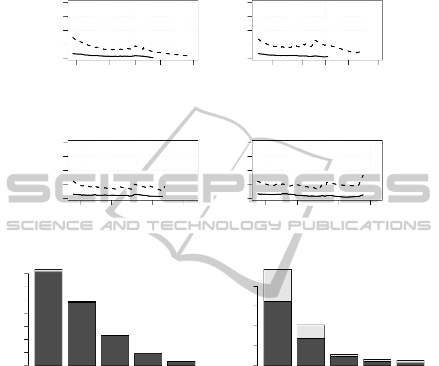
2000 5000 10000 50000

−100 0 50

SLOC

2000 5000 20000 50000

−100 0 50

C++

SLOC

1000 2000 5000 10000

−100 0 50

Java

SLOC

1000 2000 5000 10000

−100 0 50

Python

SLOC

Figure 7: Relative error in percentage for the CCDF of the lognormal and double Pareto models, compared against the CCDF

of the sample, for C, C++, Java and Python.

C C++ Java Python Lisp

% Files

0 5 10 15 20 25 30 35

Figure 8: Proportion of large and small ﬁles. The top of

the bars (clear) shows the amount of ﬁles over the threshold

values, or large ﬁles. The bottom of the bar (dark) shows

the amount of small ﬁles.

comments. It is a measure of physical size, not logical

size. For instance, if a function call in C is spawned

over several lines, it will be counted as several SLOC;

with a logical size metric, it would count only as one.

Measuring logical size is not straightforward. It

depends on the programming language. Also, there

might not be consensus about how to count some

structures like variables declaration. Should variable

declarations be counted as a logical line? And if there

is an assignation together with the declaration, should

be counted as one or two?

Coding style inﬂuences SLOC measuring. If the

coding style of a developer is to write function calls in

one line, and other developer spawns them over sev-

C C++ Java Python Lisp

% SLOC

0 10 20 30 40

Figure 9: Relative contribution of small and large ﬁles to the

overall size, for each programming language, in percentage

of SLOC. The top part of the bars (clear) is the proportion of

size due to large ﬁles. The bottom (dark) is the proportion

of size due to small ﬁles

eral lines, the second developer would appear as more

productive for the same code.

The sample under study includes code originating

from many different software projects. Therefore the

different coding styles are balanced, and the net re-

sult is representative of the actual size of the ﬁles un-

der study. However, when comparing different lan-

guages, such balance may not occur. Think for in-

stance of Lisp. Lisp syntax is based on lists, that are

represented by parentheses. Everything in Lisp is a

list: function deﬁnitions, function calls, control struc-

tures, etc. This provokes an accumulation of paren-

theses at the end of code blocks. Sometimes, for clar-

ON THE DISTRIBUTION OF SOURCE CODE FILE SIZES

(defun (m x y z)

(cond

((and (> x z) (> y z))

(+ (* x x) (* y y))

)

((and (> x y) (> z y))

(+ (* x x) (* z z))

)

(t (+ (* y y) (* z z))

)

Figure 10: Sample of code written in Lisp. Note the accu-

mulation of parentheses at the end of the blocks, resulting

in additional SLOC.

ity purposes, this parentheses are indented alone in a

new line, to match the start column of the block. Fig-

ure 10 shows an example, that will account for two

extra SLOC because of the coding style with the end-

ing parentheses. This makes the code more readable.

However, this practice will make Lisp to appear with

larger ﬁles than other languages. In general, the cod-

ing style can over represent the size of some program-

ming languages, and this may affect the shape of the

distribution.

Another threat to the validity of the results is the

sample itself. We have exclusively selected open

source, coming from only one distribution. Although

the sample is very broad and large, and the only re-

quirement for a project to be included is to be open

source, the distribution practices when adding soft-

ware to the collection may suppose a bias in the

sample. This threat to the validity can be solved

by studying other samples coming from different

sources. It can easily be tested whether the distribu-

tion with these other sources is still a double Pareto,

and whether the parameters of the distributions for

the different programming languages are different to

the values here. We have not distinguished between

different domains of application either, this is to say,

we include software that belongs to the Linux kernel,

libraries, desktop applications, etc, under the same

sample. There might be differences in the typical size

of a ﬁle for different domains of applications. How-

ever, we believe that the size distribution remains re-

gardless the domain of application. This threat to the

validity can be addressed extending this study split-

ting the sample by domain of application.

Finally, some packages may contain automatically

generated code. We have not tried to remove gener-

ated code in this study. In a similar study (Herraiz

et al., 2007), the authors showed that the inﬂuence of

very large generated ﬁles in the overall size and in the

shape of the distribution was negligible for a similar

sample, so we believe that in this case it does not af-

fect the validity of the results.

8 FURTHER WORK

The size of the sample under study makes it possible

to estimate some statistical properties of the popula-

tion from where it was extracted. In particular, the

parameters of the distribution appear to be related to

the properties of the programming language. Those

parameters could be used for software management

purposes. In this section, we discuss and speculate

about some of the possible implications of those pa-

rameters, which is clearly a line of work that deserves

further research.

The ﬁrst interesting point about the distribution of

ﬁle sizes is the difference between the two regions,

lognormal and power-law, within that distribution.

One of the parameters of the distribution, x

min

, divides

the ﬁles among small and large ﬁles. But this is much

more than a label: small ﬁles belong to a lognormal

distribution and large ﬁles to a power law distribu-

tion. In other words, that threshold value separates

ﬁles that are of a different nature, small and large ﬁles

probably will exhibit different behavior in the main-

tenance and development processes. One explanation

could be that large ﬁles are not manageable by devel-

opers, so they either are split or abandoned. If they

are split, the original ﬁle will appear as one or more

small ﬁles. If they are abandoned, then instead of an

active maintenance process, they are probably subject

of only corrective maintenance.

This transition from the small to large ﬁle is un-

conscious, developers do not split ﬁles on purpose

when they get large. However, this unconscious pro-

cess is reﬂected as a statistical property of the system.

This means that the value of this transition point can

be used as a warning threshold for software mainte-

nance. If a ﬁle gets larger than the threshold, it is

likely that it will need splitting or it will become un-

manageable.

To verify these claims we need to obtain histori-

cal data about the life of ﬁles. We must obtain the

size of ﬁles after every change during their life, fol-

lowing possible renames. If we assume that ﬁles start

empty (or with very small sizes), with that historical

information we can ﬁnd out how ﬁles grow over the

threshold size and change their nature. We can also

observe how the parameters of the distribution of size

changes over the history of the project. For instance,

the double Pareto distribution might be a character-

istic of only mature projects. Another point that de-

ICSOFT 2011 - 6th International Conference on Software and Data Technologies

Table 4: Median and threshold sizes (in SLOC), and scaling

parameter for ﬁve programming languages.

Lang. Median x

min

C 85 1, 820 2.87

C++ 58 1, 258 2.80

Java 43 846 3.17

Python 59 826 2.90

Lisp 132 1, 270 2.73

serves further work is why shell and Perl do not ex-

hibit this behavior.

The parameters of the distribution seem to be re-

lated to the programming language. Table 4 summa-

rizes the median, threshold sizes and scaling param-

eters for the ﬁve languages with a double Pareto dis-

tribution. We use medians and not average values be-

cause the distribution of size is highly right skewed,

and very large ﬁles may easily distort the average

value; the median value is more robust to very large

ﬁles.

The higher thresholds correspond to C, C++ and

Lisp. These languages also have the highest median.

This is probably due to the expressiveness of the lan-

guage (in terms of number of required lines of code

per unit of functionality). C and Lisp are the least ex-

pressive languages. In C for instance, complex data

structures are not available by default in the language,

and they have to be implemented by the developer,

or reused from a library. In Lisp, because of its sim-

ple syntax, it probably requires more lines of code to

perform the same tasks that in other languages. The

median size of Lisp ﬁles seem to support this argu-

ment.

Java and Python have the lowest thresholds. The

case of Java is interesting because the median size of a

ﬁle in Java is much lower than in C++, in spite of the

similarity between the two programming languages.

This difference is also present in the threshold val-

ues. Again, the reason may be in the rich standard

libraries that accompany Java and that are not present

in C++. The same can be said if we compare C++ and

Python. These results are similar to the tables com-

paring function points and lines of code, that were

ﬁrstly reported by Jones (Jones, 1995); higher level

(and more expressive) languages have lower number

of lines of code per function point.

In short, these threshold values can be understood

as a measurement of the maximum amount of in-

formation that can be comprehended by a developer.

Above that threshold, programmers decide to split the

ﬁle, or just abandon it because it turns unmanageable.

The values are different for different programming

languages because the same task will require more or

less lines depending on the language, but they repre-

sent the same quantity or limit value. There are of

course other factors that can inﬂuence program com-

prehension (Woodﬁeld et al., 1981), but all other fac-

tors being the same, we believe that these parameters

can be related to comprehension effort for different

programming languages.

The scaling parameter, α, is also related to the ex-

pressiveness. Its value is related to the slope of CCDF

in the large ﬁles side. Lower values of α will lead

to higher ﬁle sizes in that section. If we sort by its

value all the programming languages (see Table 4),

the most expressive language is Java, closely followed

by Python. The least expressive language is Lisp.

Lisp is a simple language in terms of syntax, and it

probably requires to write more lines of code than

in other languages to perform similar tasks. There-

fore, the scaling parameter can also be understood as

a measure of the expressiveness of the programming

language.

In short, the plan that we plan to explore as further

work are the following:

• Analysis of the evolution of ﬁles over time, to ﬁnd

out how the threshold value is related to the evo-

lution of ﬁles.

• Extend the study to large samples of other pro-

gramming languages, and divide the analysis by

domain of application, to determine whether the

features of the language are related to the values

of the parameters of the double Pareto distribu-

tion, and whether different domains exhibit dif-

ferent behaviors.

• Why some languages do not show a double Pareto

distribution?. How the evolution of ﬁles of sys-

tems written in these languages differ from double

Pareto languages?

9 CONCLUSIONS

The distribution of software source code size follows

a double Pareto. We found the double pareto charac-

teristic to hold in ﬁve of the top seven programming

languages of Debian. The languages whose size fol-

lows a double Pareto are C, C++, Java, Python and

Lisp. However, Shell and Perl behave differently.

Shell and Perl are scripting languages. In the De-

bian GNU/Linux distribution, shell and Perl are pop-

ular languages for package maintenance. The pack-

age maintenance tasks are quite repetitive, and they

are probably the same for a broad range of different

packages. So it is probably not difﬁcult to ﬁnd scripts

as part of the packages to make the packaging pro-

cess easier. Scripts are different to other kind of pro-

ON THE DISTRIBUTION OF SOURCE CODE FILE SIZES

grams: they are probably less complex and smaller.

If the difference is due to this cause, it would mean

that double Pareto distributions are the signature of

the programming process, and that different program-

ming activities (scripting, complex programs coding)

can be identiﬁed by different statistical distributions

of software size.

In any case, the double Pareto distribution already

has important practical implications for software es-

timation. Previously proposed models (Zhang et al.,

2009) are based on the lognormal distribution, that

consistently and dangerously underestimate the size

of large ﬁles. It is true that large ﬁles are only a minor-

ity in software projects, the so-called small class/ﬁle

phenomenon, however they account for a proportion

of the size as important as in the case of small ﬁles.

Therefore, using the lognormal assumption leads to

an underestimation of the size of large ﬁles. This un-

derestimation will have a great impact on the accuracy

of the estimation of the size of the overall system.

REFERENCES

Baxter, G., Frean, M., Noble, J., Rickerby, M., Smith, H.,

Visser, M., Melton, H., and Tempero, E. (2006). Un-

derstanding the shape of java software. In Proceedings

of the ACM SIGPLAN Conference on Object-Oriented

Programming Systems, Languages, and Applications,

pages 397–412, New York, NY, USA. ACM.

Boehm, B. B. (1981). Software Engineering Economics.

Prentice Hall.

Clark, D. W. and Green, C. C. (1977). An empirical study

of list structure in Lisp. Communications of the ACM,

20(2):78–87.

Clauset, A., Shalizi, C. R., and Newman, M. E. J. (2007).

Power-law distributions in empirical data.

Concas, G., Marchesi, M., Pinna, S., and Serra, N. (2007).

Power-laws in a large object oriented software sys-

tem. IEEE Transactions on Software Engineering,

33(10):687–708.

Graves, T. L., Karr, A. F., Marron, J., and Siy, H. (2000).

Predicting fault incidence using software change his-

tory. IEEE Transactions on Software Engineering,

26(7):653–661.

Halstead, M. H. (1977). Elements of Software Science. El-

sevier, New York, USA.

Herraiz, I. (2009). A statistical examination of the evo-

lution and properties of libre software. In Proceed-

ings of the 25th IEEE International Conference on

Software Maintenance (ICSM), pages 439–442. IEEE

Computer Society.

Herraiz, I., Gonzalez-Barahona, J. M., and Robles, G.

(2007). Towards a theoretical model for software

growth. In International Workshop on Mining Soft-

ware Repositories, pages 21–30, Minneapolis, MN,

USA. IEEE Computer Society.

Jones, C. (1995). Backﬁring: converting lines of code to

function points. Computer, 28(11):87 –88.

Knuth, D. E. (1971). An empirical study of FORTRAN pro-

grams. Software Practice and Experience, 1(2):105–

133.

Louridas, P., Spinellis, D., and Vlachos, V. (2008). Power

laws in software. ACM Transactions on Software En-

gineering and Methodology, 18(1).

McCabe, T. J. (1976). A complexity measure. IEEE Trans-

actions on Software Engineering, SE-2(4):308–320.

Mitzenmacher, M. (2004a). A brief history of generative

models for power law and lognormal distributions. In-

ternet Mathematics, 1(2):226–251.

Mitzenmacher, M. (2004b). Dynamic models for ﬁle sizes

and double Pareto distributions. Internet Mathemat-

ics, 1(3):305–333.

R Development Core Team (2009). R: A Language and

Environment for Statistical Computing. R Foundation

for Statistical Computing, Vienna, Austria. ISBN 3-

900051-07-0.

Robles, G., Gonzalez-Barahona, J. M., Michlmayr, M.,

Amor, J. J., and German, D. M. (2009). Macro-

level software evolution: A case study of a large soft-

ware compilation. Empirical Software Engineering,

14(3):262–285.

Robles, G., Gonzlez-Barahona, J. M., and Michlmayr, M.

(2005). Evolution of volunteer participation in libre

software projects: evidence from Debian. In Pro-

ceedings of the 1st International Conference on Open

Source Systems, pages 100–107, Genoa, Italy.

Woodﬁeld, S. N., Dunsmore, H. E., and Shen, V. Y. (1981).

The effect of modularization and comments on pro-

gram comprehension. In Proceedings of the 5th inter-

national conference on Software engineering, ICSE

’81, pages 215–223, Piscataway, NJ, USA. IEEE

Press.

Zhang, H., Tan, H. B. K., and Marchesi, M. (2009). The

distribution of program sizes and its implications: An

Eclipse case study. In Proc. of the 1st International

Symposium on Emerging Trends in Software Metrics

(ETSW 2009).

ICSOFT 2011 - 6th International Conference on Software and Data Technologies