IRTA: AN IMPROVED THRESHOLD ALGORITHM FOR REVERSE
TOP-K QUERIES
Cheng Luo
Department of Mathematics and Computer Science, Coppin State University
2500 West North Avenue, Baltimore, MD 21216, U.S.A.
Feng Yu, Wen-Chi Hou, Zhewei Jiang, Dunren Che
Computer Science Department, Southern Illinois University Carbondale, Carbondale, IL 62901, U.S.A.
Shan He
School of Economics and Management, Southwest Petroleum University, Chengdu, Sichuan 610500, China
Keywords:
Reverse top-k queries, RTA.
Abstract:
Reverse top-k queries are recently proposed to help producers (or manufacturers) predict the popularity of a
particular product. They can also help them design effective marketing strategies to advertise their products
to a target audience. This paper designs an innovative algorithm, termed IRTA (Improved Reverse top-k
Threshold Algorithm), to answer reverse top-k queries efficiently. Compared with the state-of-the-art RTA
algorithm, it further reduces the number of expensive top-k queries. Besides, it utilizes the dominance and
reverse-dominance relationships between the query product and the other products to cut down the cost of
each top-k query. Comprehensive theoretical analyses and experimental studies show that IRTA is a more
effective algorithm than RTA.
1 INTRODUCTION
With the availability of huge amount of data and the
need to support effective decision making, query pro-
cessing that results in ranked data items has attracted
much attention in the database research community
recently. A case in point is the well-studied top-k
queries (Akbarinia et al., 2007; Chang et al., 2000;
Chaudhuri and Gravano, 1999; Fagin et al., 2001;
Hristidis et al., 2001; Xin et al., 2006; Yi et al., 2003;
Zou and Chen, 2008), which return the k best data
items based on user preferences. Top-k queries can
effectively narrow down the data items that are of in-
terest to the users. Since top-k queries consider the
interesting data items only from the user’s perspec-
tive, it fails to aid producers with their decision mak-
ing. In view of this problem, Vlachou et al. (Vlachou
et al., 2010) proposed a new type of queries called
reverse top-k queries. While top-k queries help a cus-
tomer find the k best products, reverse top-k queries
can help a producer determine how many customers
will be interested in a given product.
Example 1 shows the difference between top-k
and reverse top-k queries. Considering the LCD (Liq-
uid Crystal Display) market. Assume there are five
types of LCDs on the market, of which the two most
important specifications, namely screen size and re-
fresh rate, are listed in Table 1. We further assume
there are three customers, their preferences, expressed
as weights on screen size and refresh rate, are listed
in Table 2. Note that the weights are normalized in
[0,1] and
∑
w
i
= 1. This treatment follows the related
research work (Hristidis et al., 2001; Xin et al., 2006)
and does not jeopardize generality.
Top-k queries are posted from the perspective of
a certain user (or customer). Suppose customer Bell
issues a top-2 query. This query will return the two
best LCDs that match his preference. In this case,
lcd1 and lcd4 will be returned because they have the
largest score (namely 70) for Bell’s weights.
In contrast, a reverse top-k query identifies what
user preferences make a given product their top-k
135
Luo C., Yu F., Hou W., Jiang Z., Che D. and He S..
IRTA: AN IMPROVED THRESHOLD ALGORITHM FOR REVERSE TOP-K QUERIES.
DOI: 10.5220/0003422501350140
In Proceedings of the 13th International Conference on Enterprise Information Systems (ICEIS-2011), pages 135-140
ISBN: 978-989-8425-53-9
Copyright
c
 2011 SCITEPRESS (Science and Technology Publications, Lda.)

products. Let’s consider a reverse top-2 query for
lcd1. By calculation, we know that lcd1 is the top-
2 products for customers Bell and Carl. Therefore the
query results will be two vectors that describe Bell
and Carl’s weights, namely (0.5,0.5) and (0.2,0.8). If
we issue a reverse top-2 query for lcd3. The query
will return only one vector that describes Adam’s
weights, namely (0.8,0.2). Obviously, lcd1 has a
larger group of potential buyers than lcd3.
Table 1: Specifications for LCDs.
LCD Screen Size Refresh Rate
lcd1 20 120
lcd2 30 80
lcd3 60 65
lcd4 40 100
lcd5 50 70
Table 2: Customer Preferences.
Customer Weight on Weight on
Screen Size Refresh Rate
Adam 0.8 0.2
Bell 0.5 0.5
Carl 0.2 0.8
Reverse top-k queries can not only help producers
(or manufacturers) predict the popularity of a particu-
lar product. They can also help them design effective
marketing strategies. For instance, to advertise lcd1
to Bell and Carl, and to advertise lcd3 to Adam.
Reverse top-k queries are different from reverse
nearest neighbor (RNN) queries (Korn and Muthukr-
ishnan, 2000) and reverse skyline queries (Dellis and
Seeger, 2007). Generally speaking, reverse top-k
queries provide a more generic way to identify poten-
tial interested customers(and their preferences) for a
given product. Existing research findings in the fields
of RNN and reverse skyline queries can not be applied
to reverse top-k queries.
The rest of the paper is organized as follows: Sec-
tion 2 formally define reverse top-k queries. Section
3 explains the original RTA algorithm and our IRTA
algorithm. Section 4 shows the experimental results
and concludes this paper.
2 PROBLEM STATEMENT
Consider an n dimensional data space D. A dataset S
on D has the cardinality |S| and represents the set of
products. Each product p ∈ S can be plotted on D as
a point. The n coordinates of p are (p
1
, p
2
,.. ., p
n
),
where p
i
stands for the ith attribute of p. Without
loss of generality, we assume that each product p has
non-negative, numerical attribute values. We further
assume smaller attribute values are preferred.
Top-k queries use a scoring function to determine
the rank of each product. The most commonly used
scoring function is a linear function that calculates
the weighted sum of attribute values. Each attribute
value p
i
has a corresponding weight w
i
, which indi-
cates p
i
’s relative importance to the rank. The linear
scoring function for p, denoted as f
w
(p), is defined
as: f
w
(p) =
∑
n
i=1
w
i
× p
i
.
A linear top-k query takes three parameters and
can be denoted as T OP
k
(S,w), where S is a dataset on
an n-dimensional data space, w is an n-dimensional
vector that represents a certain customer’s prefer-
ences. Formally, a top-k query can be defined as fol-
lows:
Definition 1. Given a dataset S on an n-dimensional
data space, a positive integer k and an n-dimensional
vector w, A top-k query T OP
k
(S,w) returns a set of
points P such that P ⊆ S, |P| = k, and ∀p
i
, p
j
: p
i
∈
P, p
j
/∈ P ⇒ f
w
(p
i
) ≤ f
w
(p
j
).
A reverse top-k query takes four parameters and
can be denoted by RT OP
k
(S,W, p), where S and W are
two datasets on an n-dimensional data space, where S
represents the set of products and W the set of user
preferences, respectively, and p represents a certain
product. A reverse top-k query is formally defined as
follows:
Definition 2. Given two datasets S and W on an n-
dimensional data space, a positive integer k and a
product p, A reverse top-k query RT OP
k
(S,W, p) re-
turns a set of weights
¯
W , such that ∀ ¯w
i
∈
¯
W , q ∈
TOP
k
(S, ¯w
i
).
3 THE RTA AND IRTA
ALGORITHMS
3.1 The RTA Algorithm
A naive brute force approach to answer a reverse top-
k query has to process a top-k query for each weight
vector w ∈W that represents user preferences. As pro-
cessing just a single top-k query involves non-trivial
calculations, evaluating |W | top-k queries can be pro-
hibitively expensive. The brute force approach is im-
practical when |S| or (and) |W | is (are) large.
Vlachou et al (Vlachou et al., 2010) proposed
the RTA (Reverse top-k Threshold Algorithm) to re-
duce the number of top-k evaluations. The algorithm
makes use of the calculated top-k results to deter-
mine if it is necessary to evaluate top-k queries for
ICEIS 2011 - 13th International Conference on Enterprise Information Systems
136

Figure 1: Algorithm RTA.
the remaining weight vectors. This algorithm is based
on the observations that similar weight vectors return
similar result sets for top-k queries (Hristidis et al.,
2001).
To make the RTA algorithm effective, it is essen-
tial to examine each pair of the most similar weight
vectors in order. Therefore, the weight vectors should
be ordered based on their pairwise similarity. Vla-
chou et al used cosine similarity (Tan et al., 2005) to
measure the similarity between each pair of weight
vectors. The first weight vector is most similar to the
diagonal vector of the space. Then the next vector is
most similar to its predecessor, and so on.
Figure 1 describes the RTA algorithm in pseudo-
code. Lines 1 to 3 initialize the variables. Specifi-
cally,
¯
W , which contains the result set of user pref-
erences, is initially empty and so is the buffer. The
variable threshold is initialized to infinity so that a
top-k query evaluation is always performed on the
first weight vector, which is inevitable. Lines 5
to 13 consider each weight vector w
i
in the pre-
arranged order. That is, each consecutive pair has
the largest cosine similarity. Here two notations are
used. As defined before, f
w
i
(p) is the linear scor-
ing function for p on w
i
, f
w
i
(p) =
∑
n
j=1
w
i
j
× p
j
.
max( f
w
i
(bu f f er)) is the maximum scoring function
for all the points in buffer, which means ∀p ∈ bu f f er,
max( f
w
i
(bu f f er)) ≥ f
w
i
(p). Line 6 compares f
w
i
with threshold, if f
w
i
is greater than the threshold,
it means the current w
i
under consideration can be
safely discarded without evaluating a top-k query
on it. Otherwise, line 7 evaluates the top-k query
on w
i
and put the results, which are a set of prod-
ucts, in buffer. Line 8 then compares f
w
i
(p) with
max( f
w
i
(bu f f er)), if the former is smaller, then w
i
should be included in the result set
¯
W . Line 12 update
the variable threshold by assigning it the max scoring
function for all the points in buffer on the next weight
vector w
i+1
.
The effectiveness of the RTA algorithm depends
largely on the similarity of each consecutive pair
of weight vectors. This is because the RTA algo-
rithm predicts if performing a top-k query on the next
weight vector is necessary by assuming that the top-k
products of the next weight vector are the same (or at
least very similar) to those of the current weight vec-
tor.
3.2 An RTA Example
Let’s use a two dimensional example to illustrate the
RTA algorithm. Consider the dataset S listed in ta-
ble 3 and dataset W listed in table 4. We further as-
sume k = 2 and the product p under study has the
value pair (1,1). RTA first evaluates a top-2 query
on w
1
and then assign the top-2 products, namely
p
1
and p
2
to buffer (line 7). Since f
w
1
(p) = 1 and
max( f
w
1
(bu f f er)) = 0.6, the inequality on line 8
holds, therefore w
1
is added to the result set
¯
W . On
line 12, threshold is updated to max( f
w
2
(bu f f er)) =
0.8. In the second iteration, w
2
is investigated.
On line 6, since f
w
2
(p) = 1, which is greater than
max( f
w
2
(bu f f er)) = 0.8, therefore no top-2 query
evaluation on w
2
is necessary, w
2
can be safely dis-
carded. The final result set
¯
W contains only w
1
.
Table 3: Dataset S.
S x y
p1 1.2 0
p2 0.5 0.5
p3 2 2
p4 2 3
p5 3 2
Table 4: Dataset W.
W x y
w1 0.5 0.5
w2 2/3 1/3
3.3 The IRTA Algorithm
The RTA algorithm aims to reduce the number of top-
k evaluations by considering similar user preference
vector pairs in order. We observed that the effective-
ness of the RTA algorithm can be dramatically im-
IRTA: AN IMPROVED THRESHOLD ALGORITHM FOR REVERSE TOP-K QUERIES
137

proved by incorporating two factors: 1) Taking into
consideration the dominance or reverse-dominance
relationships between the product under study p and
the products in the dataset S to reduce the cost of top-
k queries; 2) Relaxing the similarity requirement of
consecutive user preference vectors to further reduce
the number of top-k queries.
Let’s first define the dominance and reverse-
dominance relationships between two products p
1
and p
2
on a n-dimensional data space.
Definition 3. Given two products p
1
and p
2
on an n-
dimensional data space. p
1
dominates p
2
iff p
1
i
≤ p
2
i
,
for all 1 ≤ i ≤ n. Conversely, we say p
2
is dominated
by p
1
.
If p
1
dominates p
2
, then for any user preference
vector w, the value of the linear scoring function
f
w
(p
1
) is always less than or equal to f
w
(p
2
).
Table 5: Dataset S.
S x y
p1 1.6 0
p2 0.5 0.5
p3 2 2
p4 2 3
p5 3 2
p6 0 2.5
Let’s consider the dataset S listed in table 5. Again
we assume k = 2, the value pair for p is (1,1) and
the dataset W is listed in table 4. Clearly p is domi-
nated by p
2
and p dominates p
3
, p
4
and p
5
. In other
words, p
2
is a better product than p no matter which
user preference is concerned and similarly p is always
better than p
3
, p
4
, and p
5
. Therefore during a top-k
evaluation, we don’t need to consider these products
p
2
, p
3
, p
4
, and p
5
because their relationships with p
are already clear.
Figure 2 summarizes the above discussions in
pseudo-code. If we feed the dataset S listed in table
5, k = 2, and p(1, 1) to the method ChkDomiannce().
It will return
¯
k = 1, and
¯
S as shown in table 6.
Table 6: Dataset
¯
S.
¯
S x y
p1 1.6 0
p6 0 2.5
Clearly this method helps dramatically reduce the
size of the dataset S. It also reduces the k value to 1.
In practice, grid files are usually used to determine the
dominance (reverse-dominance) relationships betwe-
Figure 2: Algorithm ChkDominance.
en different grids. Interested readers are referred to
(Hou et al., 2008) for further reading.
The RTA algorithm is very restrictive in terms
of the similarity between consecutive user preference
vectors. To further help reduce the number of top-k
evaluations, we can relax this requirement by main-
taining a larger buffer. The size of the buffer is a user
customizable parameter.
Figure 3 shows the IRTA algorithm in pseudo-
code. The IRTA algorithm takes an extra parameter m,
which is a customizable positive integer representing
the buffer’s size. The symbol min
k
( f
w
i+1
(bu f f er)) on
line 12 denotes the k-th smallest value of the linear
scoring function for all the products in buffer. Intu-
itively, the larger the buffer size, the more accurate we
can compute the threshold, and the more unnecessary
top-k queries we can eliminate.
3.4 An IRTA Example
Let’s consider the dataset S listed in table 5 and W
listed in table 4. We further assume that p is (1,1),
k = 2, and m = 2. As discussed before, after line 2
in Algorithm IRTA, dataset S is updated to the set of
products listed in table 6, and k is updated to 1. Es-
sentially, the original problems is converted to a re-
verse top-1 query with a much reduced cardinality of
dataset S. On line 9, we first check w
1
(0.5,0.5). Af-
ter line 11, bu f f er will contain two products (since
m = 2), namely (1.6,0) and (0, 2.5). On line 16,
threshold is updated to 0 ×
2
3
+ 2.5 ×
1
3
=
5
6
. In
the second iteration, on line 10 we compare f
w
2
(p),
which is 1 ×
2
3
+ 1 ×
1
3
= 1 with threshold =
5
6
. Be-
ICEIS 2011 - 13th International Conference on Enterprise Information Systems
138

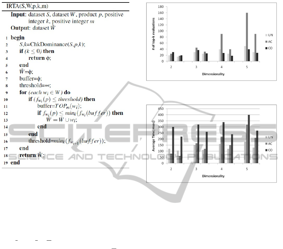
Figure 3: Algorithm IRTA.
cause f
w
2
(p) > threshold, w
2
can be safely discarded
and we don’t need to evaluate any top-k queries on
w
2
.
In contrast, if we don’t introduce m, thus we main-
tain the bu f f er with size the same as k = 1. Then
in the first iteration, on line 9, bu f f er will contain
only one value (1.6,0). On line 16, threshold =
1.6 ×
2
3
+ 0 ×
1
3
=
16
15
. In the second iteration, on line
10, we compare f
w
2
= 1 with threshold =
16
15
. Be-
cause f
w
2
< threshold, we will have to evaluate top-k
queries on w
2
.
4 EXPERIMENTAL EVALUATION
We implemented both RTA and IRTA algorithms in
Java and conducted the experiments on a computer
with 2.4GHz CPU and 1GB memory. Three synthetic
datasets, namely uniform, anti-correlated, and corre-
lated were tested. These datasets have varying dimen-
sionality from 2 to 5.
Figures 4 and 5 show the experimental results for
RTA and IRTA algorithms. For each dimensionality,
the first group of data are for RTA and the second for
IRTA. We used |S| = 10k, |W | = 10k, k = 100, and
1,000 random p’s. IRTA was shown to be able to
reduce the number of top-k queries and is thus faster
and more effective than RTA.
Figure 4: Number of top-k evaluations.
Figure 5: Average time.
REFERENCES
Akbarinia, R., Pacitti, E., and Valduriez, P. (2007). Best
position algorithm for top-k queries. Proc of VLDB,
pages 495–506.
Chang, Y.-C., Bergman, L. D., Castelli, V., Li, C.-S., Lo,
M.-L., and Smith, J. R. (2000). The onion technique:
Indexing for linear optimization queries. Proc of SIG-
MOD, pages 391–402.
Chaudhuri, S. and Gravano, L. (1999). Evaluating top-k
selection queries. Proc of VLDB, pages 397–410.
Dellis, E. and Seeger, B. (2007). Efficient computation of
reverse skyline queries. Proc of VLDB, pages 291–
302.
Fagin, R., Lotem, A., and Maor, M. (2001). Optimal ag-
gregation algorithms for middleware. Proc of PODS,
pages 102–113.
Hou, W.-C., Luo, C., Jiang, Z., and Yan, F. (2008). Approx-
imate range-sum queries over data cubes using cosine
transform. International Journal of Information Tech-
nology, 4(4):292–298.
Hristidis, V., Koudas, N., and Papakonstantinou, Y. (2001).
Prefer: A system for the efficient execution of multi-
parametric ranked queries. Proc of SIGMOD, pages
259–270.
IRTA: AN IMPROVED THRESHOLD ALGORITHM FOR REVERSE TOP-K QUERIES
139

Korn, F. and Muthukrishnan, S. (2000). Influence sets based
on reverse nearest neighbor queries. Proc of SIG-
MOD, pages 201–212.
Tan, P.-N., Steinbach, M., and Kumar, V. (2005). Introduc-
tion to data mining. Addison-Wesley, page 500.
Vlachou, A., Doulkeridis, C., Kotidis, Y., and Norvag, K.
(2010). Reverse top-k queries. Proc of ICDE, pages
365–376.
Xin, D., Cheng, C., and Han, J. (2006). Towards robust in-
dexing for ranked queries. Proc of VLDB, pages 235–
246.
Yi, K., Yu, H., Yang, J., Xia, G., and Chen, Y. (2003). Ef-
ficient maintenance of materialized top-k views. Proc
of ICDE, pages 189–200.
Zou, L. and Chen, L. (2008). Dominant graph: An efficient
indexing structure to answer top-k queries. Proc of
ICDE, pages 536–545.
ICEIS 2011 - 13th International Conference on Enterprise Information Systems
140