
LARGE-SCALE-INVARIANT TEXTURE RECOGNITION
Muhammad Rushdi and Jeffrey Ho
Computer and Information Science and Engineering, University of Florida, Gainesville, U.S.A.
Keywords:
Texture classification, Scale-invariance, Gray-level co-occurrence matrices.
Abstract:
This paper addresses the problem of texture recognition across large scale variations. Most of the exist-
ing methods for texture recognition handle only small-scale variations in test images. We propose using
microscopic-scale textures to classify texture images at any coarser scale without prior knowledge of the rel-
ative scale. In particular, given a test camera image, we compute the average error of approximating the test
texture with patches of the microscopic texture for certain category and scaling factor. Recognition is made
by selecting the category with the minimum average error over all categories and scaling factors. Experiments
on camera and low-magnification microscopic images show the validity of the proposed method.
1 INTRODUCTION
This paper explores the problem of classifying tex-
ture across large scale variations. In particular, using
high-magnification microscopic textures, we aim to
classify textures at any coarser scale. The difficulty
of the problem stems from several facts. First, im-
ages of the same material with large variations of the
imaging scale may appear so different even for a hu-
man observer (Figure 1). Second, accurate and fast
techniques need to be developed to relate the mate-
rial appearances at different scales. Although a lot
of work has been done in the area of texture recogni-
tion (Davies, 2008), (Varma and Zisserman, 2009),
little attention has been made to the effect of large
scale variations. The CUReT database (Dana and
Koenderink, 1999) captures texture images for 61 cat-
egories where each category is represented by 205 im-
ages of different viewing and illumination conditions.
However, this database lacks examples of scale vari-
ation except for 4 materials that have slightly scaled
images. Varma and Zisserman (Varma and Zisser-
man, 2009) claim that their MRF texture model is not
adversely affected by scale changes. However, their
experiments were done on the aforementioned scaled
CUReT images which have only a small scale factor
of 2. Kang (Kang and Nagahashi, 2005) developed
a framework for scale-invariant texture analysis using
multi-scale local autocorrelation features. Neverthe-
less, the experiments were limited to small changes in
scale ranging from 0.7 to 1.3. Leung and Peterson
(Leung and Peterson, 1992) used moment-invariant
and log-polar features to classify texture. However,
scale variations in their experiments were limited to
0.5, 0.67, and 1.0.
Our contribution in this paper is threefold. Firstly,
we introduce a new approach for classifying texture
across large scale variations. In particular, we show
how an approximation of a test image using micro-
scopic textures can be used to recognize textures at
any scale. Secondly, we employ our approach to es-
timate the relative scale of a test image with respect
to microscopic texture. Thirdly, we provide a dataset
of multi-scale textures that can be used to assess the
robustness of texture classifiers to scale changes.
2 COLLECTING MULTISCALE
TEXTURES
Many texture databases are freely available including
the CUReT database (Dana and Koenderink, 1999)
and the UIUC database (Lazebnik and Ponce, 2005).
While these databases sample reasonably the varia-
tions in illumination and viewing points, none of them
properly captures scale variations of the textured ma-
terials. To fill this gap, we started collecting multi-
scale texture data. In this paper, we show experiments
on five categories of materials that have challenging
textural patterns: cloth, loofa, marble, sponge, and
granite plaster (Figure 1). For every category, we
captured images using two imaging devices. Firstly,
camera texture images were collected using a high-
resolution 8-MB digital camera. Twenty images were
taken at different distances, angles and illumination
442
Rushdi M. and Ho J..
LARGE-SCALE-INVARIANT TEXTURE RECOGNITION.
DOI: 10.5220/0003398904420445
In Proceedings of the International Conference on Computer Vision Theory and Applications (VISAPP-2011), pages 442-445
ISBN: 978-989-8425-47-8
Copyright
c
2011 SCITEPRESS (Science and Technology Publications, Lda.)

Sponge
Marble
Loofa
Cloth
Plaster
Digital
Camera
Low−Magnification
Microscope
High−Magnification
Microscope
Figure 1: Multi-scale texture samples. Columns represent
images taken by a digital camera, a microscope at low and
high magnification, respectively. Each row shows images
for one type of texture.
conditions. Secondly, microscopic texture images
were collected using a low-cost hand-held digital mi-
croscope. The microscope has a magnification power
of up to 230X. However, sharp microscopic images
can be realized at magnification powers of about 60X
and 220X. For each category, we collected at least 10
images at the low-magnification level and 20 images
at the high-magnification level.
3 ALGORITHM
Our goal is to build a system that uses microscopic
textures to correctly classify textures at any coarser
scale even without prior knowledge of the relative
scale between a test image and the microscopic tex-
tures. The steps of our algorithm are as follows. First,
we create downsized versions of the microscopic im-
ages that have sizes ranging from 10× 10 pixels up
to 200 × 200 pixels (the standard size of test images
in our experiments). Second, for each of these down-
sized versions, we calculate Haralick texture features
for each of the red, green, and blue color planes as
will be explained in Section 4. Then, we store the
calculated features of the high-magnification micro-
scopic images. Third, given a test texture image, we
subdivide the image into patches of sizes correspond-
ing to those used with the microscopic images. For
each patch size selection and each candidate category,
we compute the Haralick texture features for the test
patches and find the average Euclidean distance from
the feature vector of each test patch to those of the
downsized microscopic images of the candidate cate-
gory. After that, we sum the average distance over all
the test patches. Finally, the output class for the given
test image is chosen to be the one that has the min-
imum total average distance. The minimum is taken
over all categories and all scaling factors since that
the relative scaling factor between the test image and
the microscopic images is generally unknown.
4 GRAY-LEVEL
CO-OCCURRENCE MATRICES
Interactions of neighbour pixels in texture can be de-
scribed by second-order features that are derivedfrom
the Gray-Level Co-occurrence Matrices (GLCM)
(Haralick, 1979). These matrices are defined as fol-
lows. Given a position operator P(i, j), let A be an
n× n matrix whose element A(i, j) is the number of
times that points with gray level (intensity) g
i
occur,
in the position specified by P, relative to points with
gray level g
j
. Let C be the n × n matrix that is pro-
duced by dividing A with the total number of point
pairs that satisfy P. The element C(i, j) is a measure
of the joint probability that a pair of points satisfying
P will have the values g
i
, g
j
, respectively. C is called a
co-occurrence matrix defined by P. Features derived
from such matrices exhibit high distinctive power and
relative invariance under large scale variations. We
use three of these features:
Contrast =
G−1
∑
i=0
G−1
∑
j=0
|i− j|
2
C(i, j) (1)
Energy =
G−1
∑
i=0
G−1
∑
j=0
C(i, j)
2
(2)
Homogeneity =
G−1
∑
i=0
G−1
∑
j=0
C(i, j)
1+ |i− j|
(3)
5 EXPERIMENTS AND RESULTS
5.1 Classifying Camera Images with
Fixed Scales
First, we ran the algorithm with a fixed scale. Specif-
ically, all of the high-magnification microscopic im-
ages were downsized to one fixed size and compared
LARGE-SCALE-INVARIANT TEXTURE RECOGNITION
443
with patches from the test camera image of the same
size. The recognition results for fixed sizes ranging
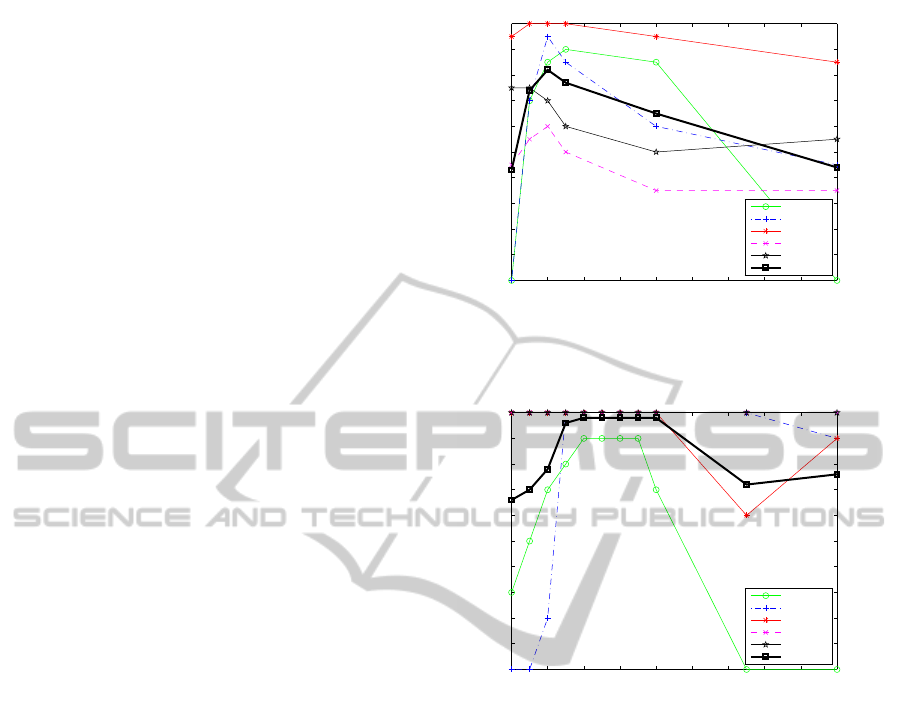
from 20× 20 to 50× 50 pixels are shown in Figure 2.
The best recognition rate of 82 % occurred at a patch
size of 40 × 40. However, the per-category perfor-
mance curves show that each material is better recog-
nized at a different scale. This suggests that we vary
the scale and let the test images choose their right rel-
ative scale.
5.2 Classifying Camera Images
with Variable Scales
As we suggested in Subsection 5.1, we ran the algo-
rithm for a range of patch sizes 10, 20, 30, 40, and 50
concurrently. The results are shown in Table 1. The
recognition rate is 82%. Despite this rate is no im-
provement over the one achieved with a fixed patch
size of 40 × 40, we still have an important advan-
tage here. In most cases, we don’t know the relative
scale difference between the test camera image and
the microscopic textures. Using our algorithm with
a variable scale will return an estimate of this scale
along with the category of the test image. For exam-
ple, of all of the 18 images of the loofa texture that
were correctly classified: 7 images were assigned a
scale of 4:1 (patch size 50× 50), 8 images were as-
signed a scale of 5:1 (patch size 40×40), and 3 image
were assigned a scale of 6.67:1 (patch size 30 × 30).
These estimated scales closely match the actual image
scales.
5.3 Classifying Low-magnification
Microscopic Textures with Fixed
Scales
To examine the ability of our algorithm to deal with
different scales, we tested the algorithm with mi-
croscopic images taken at the lower magnification
power of the microscope. Again, we ran the algo-
rithm with fixed scales. That is, all of the high-
magnification microscopic images are downsized to
one fixed size and compared with patches from the
test low-magnification microscopic image of the same
size. The recognition results for fixed sizes ranging
from 20× 20 to 200 × 200 pixels are shown in Fig-
ure 3. The best rate of 98% occurs at a patch size
ranging from 60× 60 to 90 × 90. This result is inter-
esting in two aspects. First, it makes sense to see this
improvement over the case of camera images since
the low-magnification microscopic images are closer
in scale and appearance to the high-magnification mi-
croscopic images. Second, if we compare Figures 2
20 40 60 80 100 120 140 160 180 200
0
10
20
30
40
50
60
70
80
90
100
Patch size
Classification rate
Cloth
Loofa
Marble
Sponge
Plaster
Total Rate
Figure 2: Recognition rate of test camera images as patch
size varies. The best overall rate of 82% occurs at a patch
size of 40× 40.
20 40 60 80 100 120 140 160 180 200
0
10
20
30
40
50
60
70
80
90
100
Patch size
Classification rate
Cloth
Loofa
Marble
Sponge
Plaster
Total Rate
Figure 3: Recognition rate of low-magnification micro-
scopic images as patch size varies. The best overall rate
of 98 % occurs for a range of patch sizes between 60× 60
and 90× 90.
and 3, we will notice an upward shift of the patch size
where optimal recognition rate occurs. This indeed
agrees with the intuition. Since the low-magnification
and high microscopic images are closer in scaling,
then the right scale should be smaller (i.e., the patch
size should be larger).
5.4 Classifying Low-magnification
Microscopic Textures with Variable
Scales
We retested our algorithm on the low-magnification
microscopic images after allowing the patch size to
vary from 60 × 60 to 90× 90 (the optimal patch size
range returned by the fixed-scale experiments). The
results are shown in Table 2. The overall rate is 98%
which is the same as that of the fixed-scaling exper-
iment. Again, we still get the bonus that the right
scale is returned for each test image. For example, all
VISAPP 2011 - International Conference on Computer Vision Theory and Applications
444

Table 1: Confusion matrix for classifying camera images of
Cloth (C), Loofa (L), Marble (M), Sponge (S), and Granite
Plaster (P) using high-magnification microscopic images.
The overall rate is 82%.
Material C L M S P
C 90 10 0 0 0
L 0 90 0 40 0
M 0 0 100 5 25
S 0 0 0 55 0
P 10 0 0 0 75
Table 2: Confusion matrix for classifying low-
magnification microscopic images using high-
magnification ones. The overall rate is 98%.
Material C L M S P
C 90 0 0 0 0
L 10 100 0 0 0
M 0 0 100 0 0
S 0 0 0 100 0
P 0 0 0 0 100
of the 10 images of the loofa texture were correctly
classified and additionally their estimated scales were
returned: 7 images were assigned a scale of 2.86:1
(patch size 70 × 70), 2 images were assigned a scale
of 2.5:1 (patch size 80 × 80), and 1 image was as-
signed a scale of 3.33:1 (patch size 60 × 60). These
estimated scales match roughly the actual ones.
6 CONCLUSIONS
AND FUTURE WORK
We showed in this paper how microscopic images
can be used to classify texture at coarser scales. In
the future, we plan to expand our multi-scale texture
dataset to complement the existing texture databases
and learn more about the relationship between tex-
tures at different scales.
REFERENCES
Dana, K., V.-G. B. N. S. and Koenderink, J. (1999). Re-
flectance and Texture of Real World Surfaces. ACM
Transactions on Graphics (TOG), 18(1):1–34.
Davies, E. (2008). Handbook of Texture Analysis, chap-
ter Introduction to Texture Analysis. Imperial College
Press.
Haralick, R. (1979). Statistical and structural approaches to
texture. Proceedings of the IEEE, 67(5):786–804.
Kang, Y., M.-K. and Nagahashi, H. (2005). Scale Space
and PDE Methods in Computer Vision, volume 3459,
chapter Scale Invariant Texture Analysis Using Multi-
scale Local Autocorrelation Features, pages 363–373.
Springer.
Lazebnik, S., S.-C. and Ponce, J. (2005). A sparse texture
representation using local affine regions. IEEE Trans-
actions on Pattern Analysis and Machine Intelligence,
27(8):1265–1278.
Leung, M. and Peterson, A. (1992). Scale and rotation
invariant texture classification. In The Twenty-Sixth
Asilomar Conference on Signals, Systems and Com-
puters, volume 1, pages 461–465.
Varma, M. and Zisserman, A. (2009). A statistical ap-
proach to material classification using image patch ex-
emplars. IEEE Transactions on Pattern Analysis and
Machine Intelligence, 31(11):2032–2047.
LARGE-SCALE-INVARIANT TEXTURE RECOGNITION
445
