
OPTIMAL SPATIAL ADAPTATION FOR LOCAL REGION-BASED
ACTIVE CONTOURS
An Intersection of Confidence Intervals Approach
Qing Yang and Djamal Boukerroui
Heudiasyc UMR 6599, Universit
´
e de Technologie de Compi
`
egne, Centre de Recherches de Royallieu, Compi
`
egne, France
Keywords:
Level set segmentation, Local region statistics, Intersection of confidence intervals.
Abstract:
In this paper, we propose within the level set framework a region-based segmentation method using local image
statistics. An isotropic spatial kernel is used to define locality. We use the Intersection of Confidence Intervals
(ICI) approach to define a pixel dependant local scale for the estimation of image statistics. The obtained
scale is based on estimated optimal scales, in the sense of the mean-square error of a Local Polynomials
Approximation of the observed image conditional on the current segmentation. In other words, the scale is
‘optimal’ in the sense that it gives the best trade-off between the bias and the variance of the estimates. The
proposed approach performs very well, especially on images with intensity inhomogeneities.
1 INTRODUCTION
The introduction of the level set method (Osher and
Sethian, 1988) as a general framework for segmen-
tation has overcome many of the limitations of tradi-
tional image segmentation techniques, specifically ac-
tive contours. Level set methods are parameter free,
and provide a natural approach to handle the topolog-
ical changes and the estimation of geometric proper-
ties of the evolving interface. They have become very
popular and are widely used in segmentation with
promising results (Osher and Paragois, 2003).
The use of statistical models in region-based im-
age segmentation has a long tradition. Their introduc-
tion in active contour segmentation methods, mostly
within the level set framework, led to a considerable
improvement in efficiency and robustness. For in-
stance, the CV model (Chan and Vese, 2001) and
its variant (Rousson et al., 2003) both consider im-
age background and foreground as constant intensi-
ties represented by their mean values. The mean sep-
aration method of Yezzi et al. relies on the assumption
that foreground and background regions should have
maximally different intensities (Yezzi et al., 2002).
These methods have many advantages and perform
better than edge-based models in handling the noise
and weak boundaries. However, they cannot deal
with the intensity inhomogeneities, which is almost
unavoidable in real images.
Recently, some work has been carried out in utiliz-
ing local image statistics to solve segmentation prob-
lems within the level set paradigm. A local binary
fitting method, drawn from the CV model, has been
proposed in (Li et al., 2008). A general framework
for local region-based segmentation models, with il-
lustrations on how a local energy is derived from a
global one, has been presented in (Lankton and Tan-
nenbaum, 2008). An interpretation of the piecewise
smooth Mumford-Shah functional using local Gaus-
sian models has been proposed in (Brox and Cremers,
2009). All of the above methods prove that the seg-
mentation using local statistics has the ability to cap-
ture the boundaries of inhomogeneous objects.
Local region-based segmentation models, how-
ever, are found to be more sensitive to noise than
global ones. Such models may also be more sensi-
tive to initialization if the size of the local window
is not appropriate. This brings out several problems
that need to be addressed such as: how to choose be-
tween the global and local methods to segment an im-
age? Can global and local statistics be combined in
one model? Is it possible to define a pixel dependant
local scale of the estimation of image statistics? A
first attempt within the level set framework has been
proposed in (Wang et al., 2009). Their approach is
straightforward in the sense that the proposed method
adds two energy functions of the same nature, where
the model parameters are estimated globally in one
87
Yang Q. and Boukerroui D..
OPTIMAL SPATIAL ADAPTATION FOR LOCAL REGION-BASED ACTIVE CONTOURS - An Intersection of Confidence Intervals Approach.
DOI: 10.5220/0003379100870093
In Proceedings of the International Conference on Imaging Theory and Applications and International Conference on Information Visualization Theory
and Applications (IMAGAPP-2011), pages 87-93
ISBN: 978-989-8425-46-1
Copyright
c
2011 SCITEPRESS (Science and Technology Publications, Lda.)

and locally in the other. In fact, this is not the first time
that global statistics and local statistics are combined
together to solve a segmentation problem. To our
knowledge, it is within the Bayesian framework that
the first proposition has been introduced in (Bouker-
roui et al., 1999; Boukerroui et al., 2003). The work
focused on the adaptive character of a Maximum A
Posteriori segmentation algorithm and discussed how
global and local statistics could be utilized in order
to control the adaptive properties of the segmentation
process.
Interestingly, we can learn a lot from the progress
of denoising methods (Katkovnik et al., 2010). In-
deed, traditional denoising techniques, such as filter-
ing, are based on local averaging. Therefore, their
performances depend on the number of averaged data.
An increase of the size of the averaging window do
not solve the problem as it introduces bias on im-
age regions where the noise free data are not con-
stant. In this perspective, the only possible solution
is a data dependent increase of the number of the data
or their effective weights in the filtering process. Re-
cently an interesting solution based on the Intersec-
tion of Confidence Intervals (ICI) rule has been pro-
posed. The ICI rule is used to optimise the size of
the local window in order to achieve the best trade-off
between a minimum variance and a minimum bias of
the a Local Polynomial Approximation (LPA) denois-
ing (Katkovnik et al., 2002; Katkovnik et al., 2006).
The most general formulation of the LPA-ICI method
can estimate not only the size of the local window, but
also its shape when it is used in its anisotropic form.
Motivated by the LPA-ICI method, this paper pro-
poses a segmentation method based on local statistics
with an adaptive size of local region. The size or the
scale of the local isotropic window is optimal in the
sense that it gives the best trade-off between the bias
and the variance of the estimates. This new method
provides promising segmentation results on images
with intensity inhomogeneities.
The paper is organized as follows. We briefly in-
troduce the local segmentation method in Sec. 2 and
the LPA-ICI rule in Sec. 3. In Sec. 4, we give de-
tails on the proposed method for the local ‘optimal’
scales selection and its use in the segmentation algo-
rithm. In Sec. 5, illustrative results are presented in
order to demonstrate the new development. Finally,
the authors’ conclusions are summarized in Sec. 6.
2 LOCAL REGION-BASED
SEGMENTATION METHOD
Recently, Brox and Cremers (2009) derived a sta-
tistical interpretation of the full (piecewise smooth)
Mumford-Shah functional (Mumford and Shan,
1989) by relating it to recent works on local region
statistics. They showed that the minimization of the
piecewise smooth Mumford-Shah functional is equiv-
alent to a first order approximation of a Bayesian a-
posteriori maximization based on local region statis-
tics. Precisely, it is the approximation of the Bayesian
setting with an additive noise with local Gaussian dis-
tribution, which can be expressed by the minimization
of the following energy function:
E(φ) =
Z
Ω
i
"
I(x) − µ
i
(x)
2
2σ
2
i
(x)
+
1
2
log
2πσ
2
i
(x)
#
dx
+
Z
Ω
o
"
I(x) − µ
o
(x)
2
2σ
2
o
(x)
+
1
2
log
2πσ
2
o
(x)
#
dx
+ λ
Z
Ω
δ(φ(x))|∇φ(x)|dx + ν
Z
Ω
H(φ(x))dx ,
(1)
where the subscripts ‘i’ and ‘o’ represent inside and
outside the segmentation contour C, and x are the spa-
tial positions in Ω ⊂ R
2
. The image I : Ω → R is di-
vided into foreground Ω
i
and background Ω
o
by C. H
is the Heaviside function of the level set function φ.
And the last two terms form the regularization term,
whose contribution does not depend on image statis-
tics. In Eq. (1) the local means and variances are func-
tions of the spatial position x, and can be estimated
using normalized convolutions:
µ
r
(x) =
R
Ω
K
~
(x −ζ)H
r
(φ(ζ))I(ζ)dζ
A
r
(x)
,
σ
2
r
(x) =
R
Ω
K
~
(x − ζ)H
r
(φ(ζ))(I(ζ) − µ
r
(x))
2
dζ
A
r
(x)
,
A
r
(x) =
Z
Ω
K
~
(x − ζ)H
r
(φ(ζ))dζ ,
(2)
where r = {i,o}, H
i
= H (φ(ζ)), H
o
= 1 − H (φ(ζ)).
K
~
(·) can be any appropriate local kernel, and ~ is
a scaling parameter. The minimization of Eq. (1) is
obtained when each point on the curve C has moved,
such that the local interior and local exterior of each
point along the curve are best approximated by local
means. The exact shape gradient with respect to the
level set function can be computed by the G
ˆ
ateaux
derivative. This leads to a fast implementation using
recursive filtering. More details can be found in (Brox
and Cremers, 2009, and references therein).
IMAGAPP 2011 - International Conference on Imaging Theory and Applications
88

3 ADAPTIVE WINDOW SIZE
BASED ON LPA-ICI
The LPA-ICI estimation, proposed as a nonparametric
denoising method is not as the more traditional para-
metric ones which pursue the unbiased estimation. In-
stead, it controls the value of the varying window size
in order to find a compromise between the bias and
the variance of estimation.
a) LPA Estimation. Suppose f is a function of the
spatial position x = (x,y), f (x) : R
2
→ R. We wish to
reconstruct this function using the noisy observations
I(x
s
) = f (x
s
) + ε
s
, s = 1,..., n , where the observa-
tions coordinates x
s
are known, and the ε
s
are zero-
mean random errors with variance σ
2
. Assume f can
be well approximated locally by members of a simple
class of parametric functions. Motivated by the Tay-
lor series, the LPA provides estimates in a point-wise
manner, which finds the weighted least-square fitting
in a sliding window. The standard LPA minimizes the
following criteria with respect to C:
J
h
(x) =
∑
s
w
h
(x
s
− x)
I(x
s
) − C
t
ψ
h
(x
s
− x)
2
,
where the sliding window w
h
satisfies the conven-
tional properties of kernel estimates and h is a scaling
parameter. ψ
h
is a vector of independent 2D poly-
nomials of order from 0 to m. Using an appropriate
set of polynomials, the estimate of the function f is
given as
b
f
h
(x) =
c
C
1
(x,h) and its l
th
derivative is given
by
b
C
l
(x,h) (Katkovnik et al., 2002; Katkovnik et al.,
2006). The estimate given by the LPA can be written
as the kernel operator on the observations:
b
f
h
(x) =
∑
s
g
h
(x,x
s
)I(x
s
) , (3)
where the kernel g
h
is defined by the window w
h
and the set of polynomials ψ
h
. When the grid is as-
sumed to be regular, the kernel g
h
(x,x
s
) become shift-
invariant on x and the solution is given by a convolu-
tion operation.
Assuming an additive and identically distributed
independent zero mean noise for all (local) observa-
tions, the Mean Square Error (MSE) of the LPA esti-
mate is given by (Katkovnik et al., 2002):
MSE{
b
f
h
(x,h)} = E
n
f (x) −
b
f
h
(x)
2
o
= m
2
b
f
h
(x,h) + σ
2
b
f
h
(x,h) . (4)
The analysis of MSE demonstrates that, the bias of
the estimation m
b
f
h
is a monotonically increasing func-
tion of h, while the variance σ
2
b
f
h
is a monotonically
decreasing one. This means that there exists a bias-
variance balance giving the ideal scale h
∗
, which can
be found by the minimization of Eq. (4). The ideal
scale depends, however, on the (m + 1)
th
derivative
of the unknown function f (x). The minimization of
Eq. (4) leads us to following inequalities:
|m
b
f
h
(x,h)|
≤ γ · σ
b
f
h
(x,h) if h ≤ h
∗
,
> γ · σ
b
f
h
(x,h) if h > h
∗
,
(5)
which shows that the ideal bias-variance trade-off is
achieved when the ratio between the absolute value of
the bias to the variance is equal to γ. This inequality is
the starting point for the development of a hypothesis
testing for a data driven adaptive-scale selection.
b) ICI Rule. Let h be a set of the ordered scale val-
ues h = {h
1
< h
2
< ... < h
J
}. The estimates
b
f
h
(x)
are calculated for h ∈ h and compared. The ICI rule,
which uses the estimates and their variances, iden-
tifies a scale closest to the ideal one. The estima-
tion error of the LPA satisfies the following inequality
(Katkovnik et al., 2002):
| f (x)−
b
f
h
(x)| ≤ |m
b
f
h
(x,h)| + |e
0
f
(x,h)| . (6)
Given the noise model assumptions, the random esti-
mation error, e
0
f
(x,h), follows a Gaussian probability
distribution N
0,σ
2
b
f
h
(x,h)
, where,
σ
2
b
f
h
(x,h) = σ
2
∑
s
g
2
h
(x − x
s
) .
Suppose all samples are independent to each other,
the following inequality holds with probability p =
1 − β :
|e
0
f
(x,h)| ≤ u
1−β/2
· σ
b
f
h
(x,h) , (7)
where u
1−β/2
represents the (1 − β/2)th quantile of
the normal distribution N (0,1). It means that the
values of the random error belong to the interval
with a probability p. Combining inequalities (7) and
(5), with equation (6), it can be obtained that for all
h ≤ h
∗
(Katkovnik et al., 2002):
| f (x)−
b
f
h
(x)| ≤ (γ + u
1−β/2
) · σ
b
f
h
(x,h) .
From the equations above, the confidence interval
Q(h) of the estimate is given by:
Q(h) =
h
b
f
h
(x) − Γ · σ
b
f
h
(x,h),
b
f
h
(x,h) + Γ · σ
b
f
h
(x,h)
i
.
where Γ = γ + u
1−β/2
. This is equivalent to: ∀h
i
≤
h
∗
(x), f
h
i
(x) ∈ Q(h
i
) holds with probability p. There-
fore, for all h
i
< h
∗
, the Q(h
i
) have a point in com-
mon, namely f (x). If the ICI is empty, it indicates
h
i
> h
∗
. In this way, the ICI rule can be used to test
the existence of this common point and to obtain the
adaptive window size. The ICI algorithm is defined
by the following steps:
OPTIMAL SPATIAL ADAPTATION FOR LOCAL REGION-BASED ACTIVE CONTOURS - An Intersection of
Confidence Intervals Approach
89
1. Define a sequence of confidence intervals Q
i
= Q(h
i
)
with their lower bounds L
i
and upper bounds U
i
:
L
i
=
b
f
h
i
(x) − Γ · σ
b
f
h
i
(x,h
i
) ,
U
i
=
b
f
h
i
(x) + Γ · σ
b
f
h
i
(x,h
i
) .
2. For i = 1,2,. . .,J − 1, let
L
i+1
= max{L
i
,L
i+1
}, L
1
= L
1
,
U
i+1
= min{U
i
,U
i+1
}, U
1
= U
1
.
According to these formulas, L
i+1
and U
i+1
are respec-
tively nondecreasing and nonincreasing sequences.
3. The ICI rule is finding the largest i, when L
i
≤ U
i
, i =
1,2,.. . ,J, is still satisfied.
4 PROPOSED METHOD
We propose applying the ICI approach to optimize the
spatial adaptation for local region-based active con-
tours. For each point, it finds an optimal kernel size
that meets the trade-off between the bias and the vari-
ances of estimate. This optimal local scale is then
used for the estimation of the local means and vari-
ance of the segmentation model as given in Eq. (2).
Suppose we are given a noisy image I with inten-
sity inhomogeneities within its foreground and back-
ground. We define an initial zero level set C, as the
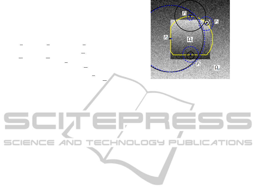
yellow contour that is shown in Fig. 1. Given a finite
set of scale values h, we calculate the g
h
for each el-
ement. Then utilize the LPA Eq. (3) to get the local
estimations of the regions inside, Ω
i
, and outside, Ω
o
,
respectively. It means that if a point x is inside of C,
its approximation uses the overlapping area of its lo-
cal kernel g
h
(x) and Ω
i
, and vice versa. As introduced
in Sec. 3, we can calculate the confidence intervals of
this estimation, then apply the ICI algorithm for each
point. After that, we obtain the optimal kernel size
that well balances the estimate bias-variance.
To find out the relation of these data adaptive
scales with the position of segmentation contour, we
picked out several typical points for analysis. As we
are only interested on a narrow band of C, within
which we select four pairs of neighbor points where
one is inside (marked with blue ‘+’) and the second
is outside (marked with black ‘◦’) the contour C (see
Fig. 1). The corresponding estimated scales are also
illustrated on the same figure with circles.
The leftmost pair P
4
lays around a region with
very low contrast between Ω
i
and Ω
o
, where the local
statistics are very similar. Also the contour near P
4
is the correct boundary. In order to maintain this par-
tition, we tend to consider more information, which
is corresponding to the larger kernel size obtained by
LPA-ICI algorithm.
Figure 1: Adaptive kernel sizes obtained by LPA-ICI algo-
rithm (image size 128 × 128, SNR = 10 dB).
For the pair P
1
around the top of C, the inside one,
lays between C and the real boundary, has small ker-
nel size. Because in that position, larger window will
introduce greater estimation bias. While its symmet-
ric point within Ω
o
has larger window, because in this
neighboring region in Ω
o
, the image is relatively ho-
mogenous. Reversely, the pairs P
2
and P
3
have larger
window inside and smaller one outside. Therefore,
if we directly use these kernel sizes in the segmenta-
tion algorithm, as the contour C gets closer to the real
boundary, the local regions of points between them
become smaller and smaller, and so will be the es-
timated local scale. It brings out the problem that
the closer C is to the correct segmentation, slower the
evolution speed is. Analyzing case P
1
(P
2
), the scale
in the inside (outside) has to be at least as bigger as
the outside (inside) in order to increase the force driv-
ing the segmentation process. To overcome this prob-
lem, one possible solution is to set a minimum scale
in h, bigger enough for a correct estimation of local
image statistics. An alternative solution is to run a
max filter, of a small size 3×3, on the estimated local
scales, so that near the contour, the estimated scales
have similar values. This filtering operation is neces-
sary only when the algorithm is in progress. Indeed,
the estimated scales, given the correct segmentation,
are very appropriate as it can be seen on the point P
4
.
Our algorithm is organized as follows:
1. Initialization. Given an image I, an initial seg-
mentation C or φ, a finite set of half window sizes
h and a vector of polynomials ψ. For each h ∈ h,
calculate the LPA kernel g
h
.
2. Optimal Spatial Kernel Size Estimation. LPA-
ICI algorithm: with g
h
, estimate the image inside
and outside of C by the LPA; apply the ICI rule on
the estimation, in order to get the adaptive window
size h
+
for this C.
3. Local Region-based Segmentation. Use the lo-
IMAGAPP 2011 - International Conference on Imaging Theory and Applications
90
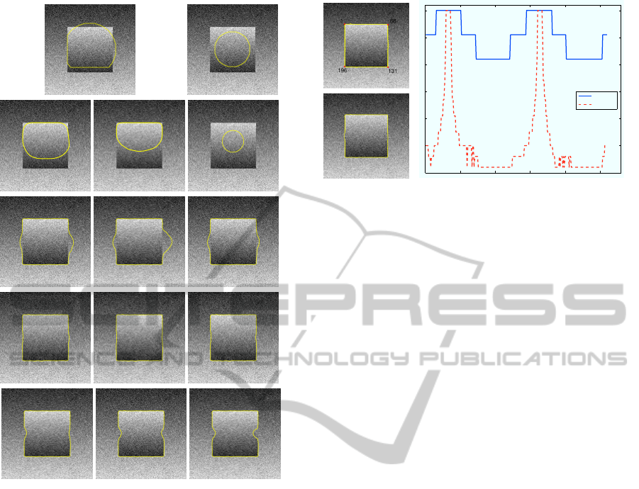
Figure 2: Segmentation results of Fig. 1 for two initializa-
tions. The top row shows the initial contours. From the 2nd
row to the bottom row using: the global CV model, local
MS method with ~ = 30, ~ = 26 and ~ = 22. Left column,
results after 100 iterations. Middle and right columns, re-
sults after 200 iterations.
cal statistics within h
+
for local piecewise smooth
MS segmentation (Brox and Cremers, 2009).
4. Repeat steps 2 and 3 until convergence.
5 EXPERIMENTS & DISCUSSION
In this section we analyze the performance of the pro-
posed segmentation algorithm and compare it with the
global and the single local scale segmentation meth-
ods. We utilize the Chan-Vese model (Chan and Vese,
2001) as a global method and the local piecewise
smooth MS method (Brox and Cremers, 2009) as a
local one. For local methods, we use a Gaussian ker-
nel with a standard deviation ~ = h
+
/3.
Fig. 2 shows the segmentation results on the syn-
thetic image of Fig. 1, obtained using the CV and
0 50 100 150 200 250
30
40
50
60
70
80
90
Outside
Inside
Figure 3: Segmentation results of the proposed method.
Left column: results for the two initializations shown in
Fig. 2. Right column: the estimated optimal spatial kernel
sizes for the left top segmentation contour, clockwise along
the contour, for the inside and the outside of C.
the local MS model for three different scales. The
CV models fails to produces correct results because
the global model supposes a constant foreground and
background. It is, therefore, inappropriate to segment
images with intensity inhomogeneities. Three differ-
ent scales are used to test and study the influence of
the kernel scale in the local MS method. As expected,
the underling model is more appropriate, as two of the
three results, obtained with the smaller kernel size,
are better than the global. Notice, however, unless
we choose an appropriate kernel scale, here around
~ = 26, the local MS model is not able to distinguish
the parts with a very low contrast between inside and
outside of C. Notice also that both methods converge
to different solutions given different initializations.
The result of the proposed scale adaptive segmen-
tation algorithm on the same test image is presented
in Fig. 3). A very satisfactory result is obtained. For
a further analysis, plots of the estimated local win-
dow sizes along the final contour, for the inside and
the outside regions, are also shown. The plots follow
a pixel clockwise parametrization of the curve start-
ing from the top left corner. Notice for example that
the estimated scales in Ω
i
are smaller than the out-
side region. This can be explained by the fact that the
inhomogeneity in Ω
i
is stronger than in Ω
o
. This dif-
ference of scales, between the inside and the outside,
is important for the forces in competition around low
contrasted boundaries. This experiment demonstrates
that local models perform better on images with in-
tensity inhomogeneities, and also that the selection of
the size of the local kernel is of a high importance in
order to achieve acceptable results.
Finally, we consider the influence of the noise
level on the estimation of the spatial kernel size. For
this experiment, we use the same synthetic image, and
study the LPA-ICI behavior on three typical pairs of
OPTIMAL SPATIAL ADAPTATION FOR LOCAL REGION-BASED ACTIVE CONTOURS - An Intersection of
Confidence Intervals Approach
91
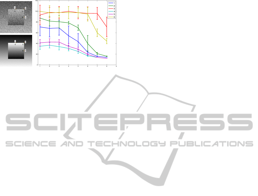
Figure 4: Adaptive scale obtained by ICI rule for the same
image with decreasing noises. Left column: test images
for SNR= 2 and SNR= 32. ‘1’,‘2’,‘3’ are points in Ω
o
;
‘4’,‘5’,‘6’ are the points in Ω
i
. Right column: estimated
kernel size error bars versus increasing SNR values for the
6 chosen points. SNR ∈ {.5,1, 2,4,8,16,25,32}. 20 values
are used for mean and variance estimation.
points (smiliar as in Fig. 1). A number in 1 to 6 is as-
signed to each point as shown in Fig. 4. The study is
carried out for the special case of an ideal segmenta-
tion (to discard the influence of bias estimation). In
order to obtain statistically meaningful estimations,
we run the experiment 20 times and for 8 different
SNR values. The means and the standard deviations,
calculated with the 20 estimated kernel sizes, are vi-
sualized as error bars versus increasing SNR values
on Fig. 4, a curve for every point.
First, we observe that the kernel size is inversely
proportional to the SNR value. Second, the variance
of the estimation is also inversely proportional to the
SNR value. These observations imply that, when the
image SNR increases, the corresponding optimal ker-
nel size decreases, and the proposed segmentation
method tends to be more local. Reversely, if the SNR
of image is small, the proposed method will adap-
tively use large kernel sizes. As expected, bigger ker-
nel sizes are obtained for the exterior points in com-
parison to their adjacent interior points. The pairs of
points ‘3’ and ‘6’ have the largest kernel estimated
sizes. Notice that for SNR values ≤ 8 dB, the ob-
tained sizes are almost equal to the maximum value
of the set h. This implies that the behavior of the
proposed method on such situation will be similar to
global methods, but locally. However, around points
‘1’ and ‘4’ the proposed method will always use local
image statistics. The curves also show that the noise
level has small influence on the estimated kernel size
at this location. This can be explained by the higher
inhomogeneity of the noise free image at this position.
In other words, the optimal scale is more governed by
the bias of the local region.
6 CONCLUSIONS
In this paper, we proposed an adaptive local region-
based segmentation method within the level set
framework. To our knowledge, this is the first work
for data driven local scale selection, in the context of
region based level set segmentation. The ICI rule is
used to derive an optimal scale for interior and exte-
rior points of the segmentation contour. The optimal-
ity is in the sense of the mean-square error minimiza-
tion of a Local Polynomials Approximation of the ob-
served image conditional on the current segmentation.
Although the presented results are preliminary, they
however, illustrate well the improvement on the state
of the art of segmentation methods. The continued
development and refinement of the proposed method,
with more experiments, should be researched in the
foreseeable future.
ACKNOWLEDGEMENTS
The authors would like to thank the Chinese Scholar-
ship Council for its financial support.
REFERENCES
Boukerroui, D., Baskurt, A., Noble, A., and Basset,
O. (2003). Segmentation of ultrasound images–
multiresolution 2D and 3D algorithm based on global
and local statistics. Pattern Recognit. Lett., 24:779–
790.
Boukerroui, D., Basset, O., Baskurt, A., and Noble, A.
(1999). Segmentation of echocardiographic data.
Multiresolution 2D and 3D algorithm based on gray
level statistics. In MICCAI, pages 516–524, Cam-
bridge, England. Springer-Verlag.
Brox, T. and Cremers, D. (2009). On local region mod-
els and a statistical interpretation of the piecewise
smooth Mumford-Shah functional. Int. J. Comput.
Vis., 84(2):184–193.
Chan, T. F. and Vese, L. A. (2001). Active contours without
edges. IEEE Trans. Image Process., 10(2):266–277.
Katkovnik, V., Egiazarian, K., and Astola, J. (2002). Adap-
tive window size image de-noising based on intersec-
tion of confidence intervals (ICI) rule. J. Math. Imag.
Vis., 16(3):223–235.
Katkovnik, V., Egiazarian, K., and Astola, J. (2006). Lo-
cal approximation techniques in signal and image pro-
cessing. The Int. Society for Optical Eng., Washing-
ton.
Katkovnik, V., Foi, A., Egiazarian, K., and Astola, J.
(2010). From local kernel to nonlocal multiple-model
image denoising. Int. J. Comput. Vis., 86:1–32.
IMAGAPP 2011 - International Conference on Imaging Theory and Applications
92

Lankton, S. and Tannenbaum, A. (2008). Localizing region-
based active contours. IEEE Trans. Image Process.,
17(11):2029–2039.
Li, C., Kao, C.-Y., Gore, J. C., and Ding, Z. (2008).
Minimization of region-scalable fitting energy for
image segmentation. IEEE Trans. Image Process.,
17(10):1940–1949.
Mumford, D. and Shan, J. (1989). Optimal approximations
by piecewise smooth functions and associated varia-
tional problems. Communications on Pure and Ap-
plied Mathematics, 42:577–685.
Osher, S. and Paragois, N. (2003). Geometric level set meth-
ods in imaging vision and graphics. Springer Verlag.
Osher, S. and Sethian, J. A. (1988). Fronts propagating
with curvature-dependent speed: Algorithms based
on Hamilton-Jacobi formulations. J. Comput. Phys.,
79(1):12–49.
Rousson, M., Brox, T., and Deriche, R. (2003). Active un-
supervised texture segmentation on a diffusion based
feature space. Technical Report 4695, INRIA.
Wang, L., Li, C., Sun, Q., Xia, D., and Kao, C.-Y. (2009).
Active contours driven by local and global inten-
sity fitting energy with application to brain MR im-
age segmentation. Comput. Med. Imaging Graph.,
33(7):520–531.
Yezzi, A., Tsai, A., and Willsky, A. (2002). A fully global
approach to image segmentation via coupled curve
evolution equations. J. Visual Communication Image
Representation, 13(1-2):195–216.
OPTIMAL SPATIAL ADAPTATION FOR LOCAL REGION-BASED ACTIVE CONTOURS - An Intersection of
Confidence Intervals Approach
93
