
BIOLOGICALLY INSPIRED ROBOT NAVIGATION BY
EXPLOITING OPTICAL FLOW PATTERNS
Sotirios Ch. Diamantas
∗
Intelligence, Agents, Multimedia Group, School of Electronics and Computer Science
University of Southampton, Southampton, SO17 1BJ, U.K.
Anastasios Oikonomidis
Centre for Risk Research, School of Management, University of Southampton, Southampton, SO17 1BJ, U.K.
Richard M. Crowder
Intelligence, Agents, Multimedia Group, School of Electronics and Computer Science
University of Southampton, Southampton, SO17 1BJ, U.K.
Keywords:
Optical flow, Biologically inspired robot navigation, Robot homing, Visual navigation, Mobile robotics.
Abstract:
In this paper a novel biologically inspired method is addressed for the robot homing problem where a robot
returns to its home position after having explored an a priori unknown environment. The method exploits
the optical flow patterns of the landmarks and based on a training data set a probability is inferred between
the current snapshot and the snapshots stored in memory. Optical flow, which is not a property of landmarks
like color, shape, and size but a property of the camera motion, is used for navigating a robot back to its home
position. In addition, optical flow is the only information provided to the system while parameters like position
and velocity of the robot are not known. Our method proves to be effective even when the snapshots of the
landmarks have been taken from varying distances and velocities.
1 INTRODUCTION
Recently there has been a resurgence of interest in
biologically inspired robotics. Biology is seen as an
alternative solution to the problems robots encounter
which includes algorithmic complexity, performance,
and power consumption among others. The num-
ber of neurons an insect possess is approximately
10
6
while those found in a human brain are between
10
10
and 10
11
. Biological inspiration provides simple,
yet effective methods for the solutions of such prob-
lems. The careful examination of those methods has a
twofold gain. By examining the methods animals em-
ploy we can design better and more efficient robots,
and by building such robots we can understand better
how the mechanisms of animals work as well as how
they have evolved over time.
∗
Currently a postdoctoral research associate within In-
telligent Robot Lab, Pusan National University, Republic
of Korea.
Navigation lies at the heart of mobile robotics.
Homing (or inbound journey) refers to the navigation
process where an autonomous agent performs a return
to its home position after having completed foraging
(or outbound journey; foraging is mainly attributed to
a biological agent). A robot may have to return to its
base for a number of reasons like recharging batter-
ies, failure of a subsystem, or completion of a task.
The application areas of robots capable of performing
homing are plenty and vary. Search and rescue robots
are in need in areas that have been hit by earthquakes
or in environments which are hazardous for humans
(Matsuno and Tadokoro, 2004). Planetary missions
to other regions constitute another application area
of robots whose navigation process involves returning
back to their base. In this paper we have developed a
novel approach to tackle the problem of robot homing
using visual modality as the only source of informa-
tion. No other sensor is provided to the robotic agent
apart from two side cameras mounted on a simulated
645
Ch. Diamantas S., Oikonomidis A. and M. Crowder R..
BIOLOGICALLY INSPIRED ROBOT NAVIGATION BY EXPLOITING OPTICAL FLOW PATTERNS.
DOI: 10.5220/0003377706450652
In Proceedings of the International Conference on Computer Vision Theory and Applications (VISAPP-2011), pages 645-652
ISBN: 978-989-8425-47-8
Copyright
c
2011 SCITEPRESS (Science and Technology Publications, Lda.)

mobile platform.
Optical flow, that is the rate of change of image
motion in the retina or a visual sensor, is extracted
from the motion of an autonomous agent. The orien-
tation of the cameras on the robotic platform is per-
pendicular to the direction of motion so as a transla-
tional optical flow information is generated. Optical
flow, which is not a property of the landmarks, like
color, shape, and size, but of the camera motion has
been used for building topological maps in a priori
unknown environment based on the optical flow pat-
terns of the landmarks. The novelty of our method
lies in the fact that no information is given such as
the position or the velocity of the robot but only the
optical flow ‘fingerprint’ of the landmarks caused by
the motion of the robot. For this purpose, a train-
ing algorithm has been deployed and a probability is
inferred that is computed from the similarity of the
optical flow patterns between the maps built during
the outbound and inbound trip. The work in this pa-
per builds upon the work of (Diamantas et al., 2010)
that also appears by (Diamantas, 2010) where a single
vector was modeled at varying distances and veloci-
ties. In the current work, the optical flow pattern of a
landmark is modeled and its variation at varying dis-
tances and velocities is observed.
This paper is comprised of five sections. Follow-
ing is Section 2 where related work is presented. In
Section 3 the methodology of the homing model is de-
scribed. Section 4 presents the results of the statistical
model on the homing process of navigation. Finally,
Section 5 epitomizes the paper with a brief discussion
on the conclusions drawn from this work.
2 RELATED WORK
A large number of insects use optic flow for navi-
gation. Insects like Drosophila use the apparent vi-
sual motion of objects to supply information about
the three-dimensional structure of the environment.
The fly Drosophila uses optic flow to pick near tar-
gets. (Collett, 2002) shows that the task of evaluat-
ing distances between objects is made easier by mak-
ing side-to-side movements of the head strictly trans-
lational and disregarding any rotational components
that can influence the distance to the objects. Loom-
ing, i.e., image expansion, can also distort the actual
distance to the object as the apparent size compared
to the physical size of the object differs. In his exper-
iments (Collett, 2002) ascertains that Drosophila like
many insects limit rotational flow during exploratory
locomotion. In fact, Drosophila move in straight-line
segments and restrict any rotation to saccades at the
end of each segment. (Schuster et al., 2002) have used
virtual reality techniques to show that fruit flies use
translational motion for picking up the nearest object
while disregarding looming.
Ladybirds also move in straight-line segments and
rely on translational optic flow rather that looming
cues. Other animals like locusts and mantids turn
their head from one side to the other just before jump-
ing. (Kral and Poteser, 1997) suggest that locusts and
mantids use translational motion to infer the three-
dimensional structure of the environment and in par-
ticular the distance to the object they wish to ap-
proach. In some other experiments performed by
(Tautz et al., 2004) trained bees had to travel large dis-
tances across various scenes that included both land
and water. The results showed that the flights over
water had a significantly flatter slope than the ones
above land. This suggests that the perception of the
distance covered by bees is not absolute but scene-
dependent where the optic flow perceived is evidently
larger. This may also suggest why some bees are
drowning by ‘diving’ into lakes or the sea while fly-
ing above water. The distance and direction to a food
source is communicated in the bees by means of wag-
gle dances that integrate retinal image flow along the
flight path (Esch et al., 2001), (von Frisch, 1993).
Experiments conducted by (Hafner, 2004) have
shown that in principle visual homing strategies can
be both learnt and evolved by artificial agents. Even
a sparse topological representation of place cells can
lead to good spatial representation of the environment
where metric information can easily be extracted, if
required, by the agent. Nevertheless, it is not clear
which navigation strategy is applied by an animal,
since its behavior consists of a combination of dif-
ferent strategies. When, and to what extent, the dif-
ferent strategies are chosen and which sensory modal-
ities are applied is still an open question. Two well-
known homing models are the snapshot and the Av-
erage Landmark Vector (ALV) model. The snapshot
model is an implementation of the template hypoth-
esis (Cartwright and Collett, 1983; Cartwright and
Collett, 1987). It requires a panoramic snapshot of
the goal position, be it a hive, nest, or a food source.
Along with the snapshot the compass direction is
stored. The snapshot model is an image matching pro-
cess between a snapshot taken at a goal position and a
snapshot containing the current view. The image ob-
tained from the omnidirectional camera is unwrapped
and a threshold operation is performed to yield a one-
dimensional black and white image. The landmarks
are denoted as black marks on the image. Then, this
is compared with the snapshot of the current view
to produce the homing vector. The homing vector is
VISAPP 2011 - International Conference on Computer Vision Theory and Applications
646

a two-dimensional vector pointing towards the home
position, and is obtained by summing up all radial and
tangential vector components.
The ALV model developed by (Lambrinos et al.,
2000) uses, too, a processed panoramic image but, in
contrast to the snapshot model, it need not be stored.
Only a two-dimensional vector for each landmark
needs to be stored that points to the direction of the
landmark. Matching and unwrapping of the image are
not required, since the calculations are performed on
the basis of vector components. Thus, ALV is more
parsimonious than the snapshot model. Nevertheless,
snapshots in the ALV model have to be captured and
processed to produce a one-dimensional picture, as is
in the snapshot model. An application of a robot with
homing abilities using panoramic vision is demon-
strated by (Argyros et al., 2005).
2.1 Applications of Optical Flow
Lately a growing number of autonomous vehicles
have been built using techniques inspired by insects
and, in particular, optic flow. One of the first works
that studied the relation of scene geometry and the
motion of the observer was by (Gibson, 1974). A
large amount of work, however, has been focused on
obstacle avoidance using optical flow (Camus et al.,
1996; Warren and Fajen, 2004; Merrell et al., 2004).
The technique, generally, works by splitting the im-
age (for single camera systems) into left- and right-
hand side. If the summation of vectors of either side
exceeds a given threshold then the vehicle is about
to collide with an object. Similarly, this method has
been used for centering autonomous robots in cor-
ridors or even a canyon (Hrabar et al., 2005) with
the difference that the summation of vectors this time
must be equal in both the left-hand side and the right-
hand side of the image. (Ohnishi and Imiya, 2007)
utilize optical flow for both obstacle avoidance and
corridor navigation. The performance of optical flow
has also been tested in underwater color images by
(Madjidi and Negahdaripour, 2006). (Vardy, 2005)
employs various optical flow techniques that are com-
pared using block matching and differential methods
to tackle homing. In a recent work implemented by
(Kendoul et al., 2009) optic flow is used for fully
autonomous flight control of an aerial vehicle. The
distance travelled in this Unmanned Aerial Vehicle
(UAV) is calculated by integrating the optical flow
over time. A similar work for controlling a small
UAV in confined and cluttered environments has also
been implemented by (Zufferey et al., 2008). (Bar-
ron et al., 1994) discuss the performance of optical
flow techniques. Their comparison is focused on ac-
curacy, reliability and density of the velocity measure-
ments. Other works employ optic flow methods for
depth perception (Simpson, 1993), motion segmenta-
tion (Blackburn and Nguyen, 1995), or estimation of
ego-motion (Frenz and Lappe, 2005).
A similar technique to optical flow developed by
(Langer and Mann, 2003) called optical snow arises
in situations where camera motion occurs in highly
cluttered 3D environments. Such cases involve a pas-
sive observer watching the fall of the snow, hence the
name of the method optical snow. Optical snow has
been inspired by research in animals that inhabit in
highly dense and cluttered environments; such ani-
mals include the rabbit, the cat, and the bird. The
properties of the optical snow are that yields dense
motion parallax with many depth discontinuities oc-
curring in almost all image points. This comes in
contrast to the classical methods that compute opti-
cal flow and presuppose temporal persistence and spa-
tial coherence. (Langer and Mann, 2003) present the
properties of optical snow in the Fourier domain and
investigateits computational problems on motion pro-
cessing.
3 METHODOLOGY
This section is dedicated to the description of the op-
tical flow method. It is described how the optical flow
‘signature’ of the landmarks, that is caused by the per-
ceived motion of the robot in the environment, can be
used to localize the robot during the homing process.
Various landmarks have been modeled and simulated
from which the robot passes through. The simulated
landmarks have geometrical shapes and they are tex-
tured in order to produce large amounts of optic flow
(as is in real environments). In this work we have
employed the Lucas-Kanade (LK) algorithm (Lucas
and Kanade, 1981). In order for the optic flow al-
gorithm to perform well images that have high tex-
ture and contain a multitude of corners are essential.
Such images have strong derivatives and, when two
orthogonal derivatives are observed then this feature
may be unique, and thus, good for tracking. Track-
ing a feature refers to the ability of finding a fea-
ture of interest from one frame to a subsequent one.
Tracking the motion of an object can give the flow
of the motion of the objects among different frames.
In Lucas-Kanade algorithm corners are more suitable
than edges for tracking as they contain more informa-
tion. For the implementation of the LK algorithm the
(OpenCV, 2008) library has been used.
As mentioned in Section I the simulated robot
consists of two side-ways cameras which are perpen-
BIOLOGICALLY INSPIRED ROBOT NAVIGATION BY EXPLOITING OPTICAL FLOW PATTERNS
647

dicular to the direction of motion. This creates a
translational optic flow as the robot navigates through
the environment. Every landmark in the environment
‘emits’ a number of optic flow vectors that are de-
pendent on the distance between the robot and the
landmark, and the velocity of the robot. One of the
advantages of our method is that the images are only
captured and are not used for storage or comparison.
Comparing and storing only the properties of vectors
between different frames reduces the computational
complexity and the cost of the homing process.
During the outbound trip of the robot the camera
detects and records the optic flow that is generated by
the motion of the vehicle. During that phase the robot
builds a topological map from the optical flow ‘fin-
gerprint’ of the landmarks. After the foraging trip,
has completed, the homing trip is initiated. In the
homing phase, the robot compares the optical flow
patterns it currently perceives with the ones occurred
during the foraging journey. If the similarity score
(i.e., probability) between the two patterns is above
a given threshold, then the robot assumes the current
landmark observed is the same with the landmark oc-
curred during the outbound trip. This information is
then used to localize the robot within the topological
map. The similarity score of the vectors is a proba-
bilistic result of the Euclidean distance of the vectors
between the current image and the image taken during
the outbound journey.
In order for the robot to localize in the environ-
ment using optic flow vectors, a training data set of
n = 1000 observations has been implemented where
the optical flow pattern of a landmark is observed at
varying distances between the robot and the landmark
and at varying velocities. These distances and the ve-
locities chosen to create the training data set approx-
imate the real distributions of velocity and distance
when a robot navigates in an environment. Thus, a
joint probability distribution has been created with
two continuousand independent variables, that is, dis-
tance and velocity, and is expressed by (1),
f
C,D
(c,d) = f
C
(c) · f
D
(d) ∀c,d. (1)
The velocity, C, and the distance variable, D, have
been drawn by two Gaussian distributions with µ =
4,σ = 1 and µ = 11, σ = 3 respectively. The n ob-
servations model the position of the landmark in the
plane under n varying distances and velocities. One
assumption that needs to be met in our method is that
the majority of the vectors comprising a given land-
mark should have the same, or almost the same mag-
nitude. In order to solve the matching problem be-
tween landmarks, the mean (or center) point of ev-
ery vector is taken. Thus, summing up all the mean
points of the vectors and dividing by the number of
vectors, v, that comprise a landmark we end up hav-
ing the mean of the means as shown in (2).
¯x, ¯y =
1
v
·
v
∑
l=1
x
l
,y
l
(2)
The mean of the means in an optical flow pattern can
be visualized as the center of gravity in a physical sys-
tem. The same process is repeated ntimes where the
center of gravity is observed at varying distances and
velocities as shown in (3). We then compute the Eu-
clidean distances between the center of gravity of all
n observations and the center of gravity of each and
every observation. Equation (4) shows the process of
finding the Euclidian distances.
x
m
,y
m
=
1
n
·
n
∑
k=1
x
k
,y
k
n = 1000 (3)
d
k
=
q
(x
m
− ¯x
k
)
2
+ (y
m
− ¯y
k
)
2
(4)
The histogram produced by the Euclidean distances,
d
k
, forms a log-normal probability density function
(pdf) with µ = 1.20 and σ = 0.71 in the log-normal
scale. In order to calculate the expected mean, E(µ),
and standard deviation, E(s.d.), the (5) and (6) should
be used, respectively.
E(µ) = e
µ+
1
2
σ
2
(5)
E(s.d.) = e
µ+
1
2
σ
2
p
e
σ
2
−1 (6)
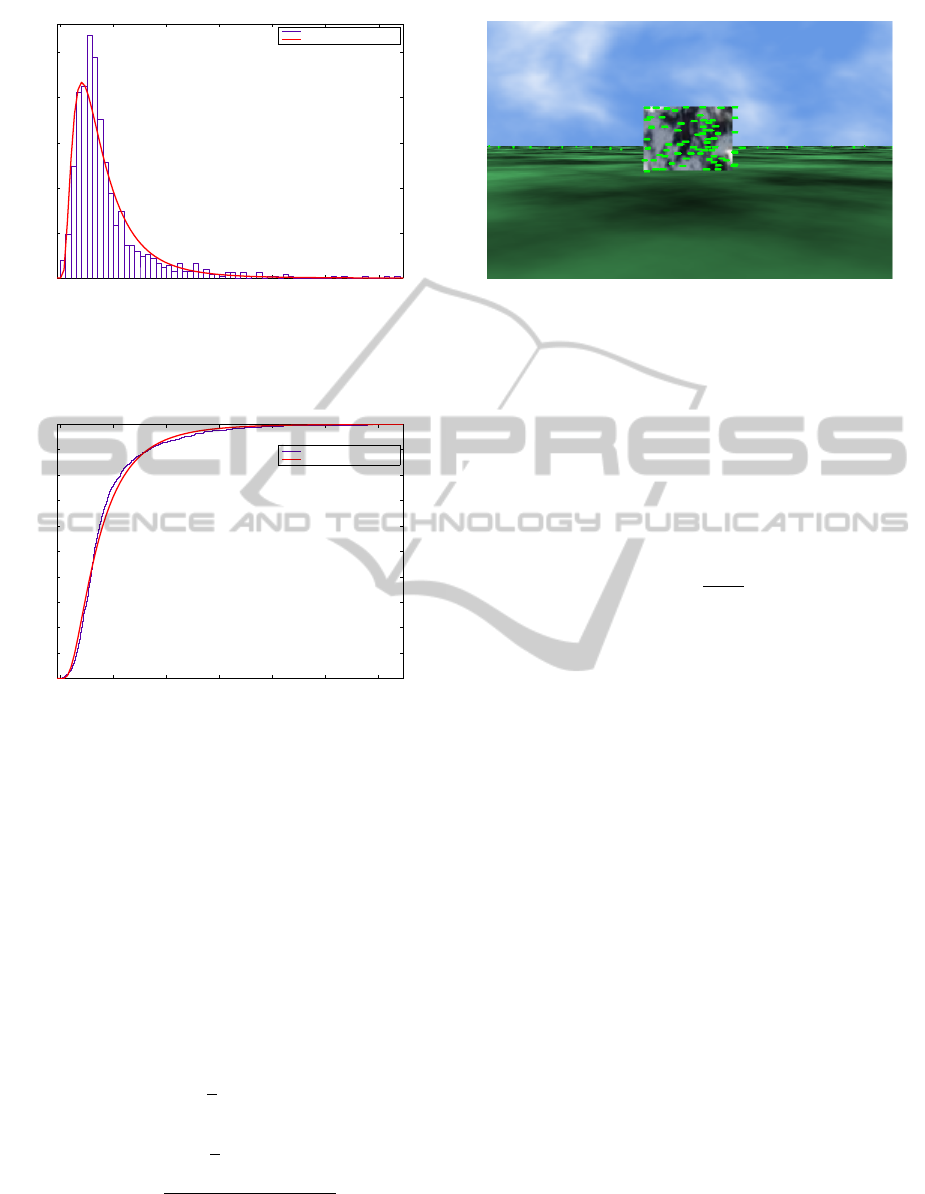
Figure 1 shows the histogram of center of gravity de-
viations and the probability density function of the
log-normal. The log-normal pdf is deployed in order
to infer the probability a match to occur between the
optical flow pattern of the current image and the op-
tical flow pattern stored in memory. Figure 2 depicts
the cumulative distribution function (cdf) of center of
gravity deviations and the log-normal. The probabil-
ity density function of log-normal is given by (7), and
the cumulative density function of log-normal is ex-
pressed by (8), where erfc is the complementary error
function and Φ is the standard normal cdf.
f
X
= (δ;µ,σ) =
1
δσ
√
2π
e
−
(lnδ−µ)
2
2σ
2
δ > 0. (7)
F
X
(δ;µ,σ) =
1
2
er fc
−
lnδ−µ
σ
√
2
= Φ
lnδ−µ
σ
(8)
Thus far we have explained the methodology of the
training algorithm. We now move on to the process
of calculating a probability for the patterns observed
VISAPP 2011 - International Conference on Computer Vision Theory and Applications
648
0 5 10 15 20 25 30
0
0.05
0.1
0.15
0.2
0.25
Data
Density
deviation of mean vector positions
log−normal pdf
Figure 1: Histogram of center of gravity deviations of the
training algorithm and the log-normal probability density
function (pdf) fit. Mean and standard deviation are µ = 1.20
and σ = 0.71 in the log-normal scale, respectively.
0 5 10 15 20 25 30
0
0.1
0.2
0.3
0.4
0.5
0.6
0.7
0.8
0.9
1
Data
Cumulative probability
deviation of mean vector positions
log−normal cdf
Figure 2: Cumulative density functions (cdf) of center of
gravity deviations and the log-normal distribution.
by the robot during the foraging and homing process.
This probability will aid the robot localize itself in the
environment. During the homing navigation process,
the robot calculates the mean of the means (center
of gravity) from every landmark and finds their Eu-
clidean distance δ with the mean of the means of the
landmarks stored in the database. Equations (9), (10),
and (11) describe the process with two distinct land-
marks. In (9), (10), n and s are the number of vectors
for two distinct landmarks i and j, one of which oc-
curs in the outbound trip while the other one occurs
in the inbound trip.
¯x
i
, ¯y
i
=
1
n
·
n
∑
a=1
x
a
,y
a
(9)
¯x
j
, ¯y
j
=
1
s
·
s
∑
b=1
x
b
,y
b
(10)
δ =
q
( ¯x
i
− ¯x
j
)
2
+ ( ¯y
i
− ¯y
j
)
2
(11)
P = 1−P
δ
(12)
Figure 3: Reference landmark and its optical flow pattern
taken at a distance of 11m and a velocity of 4km/h. This ref-
erence landmark was used for comparison with other land-
marks.
The log-normal cdf then gives us the probability P
δ
based on the Euclidean distance δ between the two
mean of the means. It is then subtracted from 1 to give
the probability P as in (12). In addition the probability
P of the log-normal is multiplied by the ratio of the
number of the vectors as shown in (13),
P
T
= P
min
i
max
j
(13)
with min
i
being the landmark i with the minimum
number of vectors and max
j
the maximum number of
vectors of landmark j. Thus, even if the Euclidean dis-
tance between the two optical flow patterns is small,
the total probability, P
T
, can be low if the ratio of the
vectors is small. Thus, two patterns which are totally
different may have a small Euclidean distance that
yields a high probability P. Multiplying this proba-
bility value by the ratio of the number of vectors can
drop significantly the total probability value, P
T
, as-
suming that the numbers of vectors are not of the same
magnitude. The landmark of Fig. 3 acts as a reference
for the following snapshots in order to demonstrate
the similarity score at different distances and veloci-
ties, and between different landmarks. The optic flow
images are produced by calculating the motion of a
landmark at two time contiguous frames. It should
also be noted that the flow vectors appear upside down
since the images are read from top to bottom.
4 RESULTS
The homing model described in this paper has been
implemented in the C++ programming language and
the (MATLAB, 2007) software was used for the anal-
ysis of the data. The breve simulator was used for the
development of the 3D environment (Klein, 2002).
BIOLOGICALLY INSPIRED ROBOT NAVIGATION BY EXPLOITING OPTICAL FLOW PATTERNS
649
0 100 200 300 400 500 600
0
50
100
150
200
250
x
y
Red elem: 113, Blue elem: 84, Divergence: 2.53, Probability: 48.52%
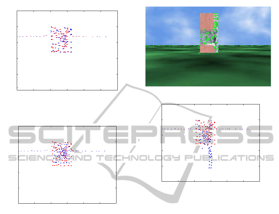
(a) Optical flow pattern of the reference landmark taken at a dis-
tance of 11m and a velocity of 3km/h.
0 100 200 300 400 500 600
0
50
100
150
200
250
x
y
Red elem: 113, Blue elem: 100, Divergence: 1.19, Probability: 82.04%
(b) Optical flow pattern of the reference landmark taken at a dis-
tance of 14m and a velocity of 4km/h.
Figure 4: Optical flow patterns of the reference landmark
taken at different distances and velocities.
The graphs of Fig. 4 demonstrate the effectiveness of
our approach by comparing the optical flow patterns
of the reference image, Fig. 3, taken at a distance
of 11m and a velocity of 4km/h with the optical flow
patterns of the same landmark but taken at varying
distances and velocities.
The circle in the graphs represents the mean po-
sition of all the vectors that comprise a landmark, in
other words the center of gravity. The red optic flow
vectors refer to the reference image while the blue
ones refer to the current snapshot. Vectors whose
length falls below a threshold (in this case 1) are con-
sidered as outliers. Divergence is the Euclidean dis-
tance between the mean position of the vectors of the
current snapshot with the mean position of the vec-
tors of the reference image. The number of elements
in the current snapshot differs from frame to frame as
the angle of perception changes. From these graphs it
is clear that the similarity score is quite high in both
(a) Tower-like landmark.
0 100 200 300 400 500 600
0
50
100
150
200
250
x
y
Red elem: 113, Blue elem: 99, Divergence: 30.77, Probability: 0.07%
(b) Optic flow patterns between the tower-like landmark and the
reference landmark.
Figure 5: Comparison of optic flow patterns between a
tower-like landmark and the reference landmark. The dis-
tance of 11m remains the same as in the reference landmark
as well as the velocity taken, that is 4km/h.
figures revealing that the same landmark has been
observed when comparing the optical flow maps be-
tween the foraging and homing process. Based on this
result the robot is able to localize itself using optical
flow maps.
Figure 5 depicts a tower-like landmark and the
reference landmark of Fig. 3. The distance and ve-
locity at which they were captured remains the same
as in the reference image, that is 11m for distance
and 4km/h for velocity. In the graph of Fig. Please
place \label after \caption, the similarity score
is quite low, that is 0.07% while the divergence is
quite high, that is 30.77. This low probability reveals
that the two landmarks are different to each other.
Finally, in Fig. 6 a pyramid-like landmark is
shown against the optical flow pattern of the reference
landmark. In this case, too, the distance and velocity
have been kept the same as in the reference landmark.
The probability in Fig. Please place \label after
\caption is low, too, that is 4.99% while the di-
VISAPP 2011 - International Conference on Computer Vision Theory and Applications
650
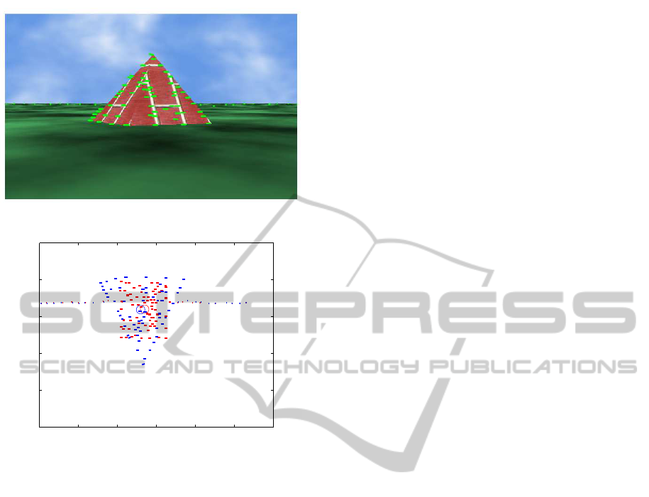
(a) Pyramid-like landmark.
0 100 200 300 400 500 600
0
50
100
150
200
250
x
y
Red elem: 113, Blue elem: 99, Divergence: 10.21, Probability: 4.99%
(b) Optic flow patterns between the pyramid-like landmark and the
reference landmark.
Figure 6: Comparison of optic flow patterns between a
pyramid-like landmark and the reference landmark. The
distance of 11m remains the same as in the reference land-
mark as well as the velocity taken, that is 4km/h.
vergence between the centers of gravity is equal to
10.21. As in the previous example, the low proba-
bilistic score reveals the dissimilarity of the two land-
marks, even though the distance and the velocity that
the images were captured are the same as in the refer-
ence landmark. It is, however, likely that two dissim-
ilar landmarks may produce a high similarity score.
This can be the case when two landmarks have simi-
lar properties such as texture, shape, and size. In such
a scenario the robot will localize itself inaccurately.
5 CONCLUSIONS
In this paper we presented a novel biologically in-
spired method to tackle the robot homing problem.
In this approach, we have considered only the opti-
cal flow patterns of the landmarks. The simulation
results show that optical flow can be used as a means
to perform homing. This method is parsimonious as
no other information is taken into account such as
position and velocity of the robot. In addition, our
method is computationally efficient as images need
not be stored but the properties of the vectors, that is
the mean of the means of the vectors and the number
of vectors in a snapshot.
Finally, comparing the current method with the
method presented by (Diamantas et al., 2010) we can
infer that the method presented in this paper is more
robust and accurate. In the method of (Diamantas
et al., 2010) the log-normal distribution has a µ = 2.24
and σ = 0.86 whereas in the current work mean and
standard deviation are µ = 1.20 and σ = 0.71, respec-
tively. This biological approach may also help explain
the methods employed by insects, and in particular
honeybees, to perform localization and thus homing.
To support this, a recent study by (Avargues-Weber
et al., 2009) reveals that honeybees are capable of dis-
criminating faces. It could well be the case of optical
flow patterns.
ACKNOWLEDGEMENTS
The authors would like to thank Dr Klaus-Peter Za-
uner for his guidance and help in shaping the optic
flow idea.
REFERENCES
Argyros, A. A., Bekris, C., Orphanoudakis, S. C., and
Kavraki, L. E. (2005). Robot homing by exploiting
panoramic vision. Journal of Autonomous Robots,
19(1):7–25.
Avargues-Weber, A., Portelli, G., Benard, J., Dyer, A., and
Giurfa, M. (2009). Configural processing enables
discrimination and categorization of face-like stim-
uli in honeybees. Journal of Experimental Biology,
213(4):593–601.
Barron, J. L., Fleet, D. J., and Beauchemin, S. S. (1994).
Performance of optical flow techniques. International
Journal of Computer Vision, 12(1):43–77.
Blackburn, M. and Nguyen, H. (1995). Vision based au-
tonomous robot navigation: Motion segmentation.
In Proceedings for the Dedicated Conference on
Robotics, Motion, and Machine Vision in the Automo-
tive Industries, pages 353–360, Stuttgart, Germany.
Camus, T., Coombs, D., Herman, M., and Hong, T.-S.
(1996). Real-time single-workstation obstacle avoid-
ance using only wide-field flow divergence. In Pro-
ceedings of the 13th International Conference on Pat-
tern Recognition, volume 3.
Cartwright, B. and Collett, T. S. (1987). Landmark maps for
honeybees. Biological Cybernetics, 57(1–2):85–93.
BIOLOGICALLY INSPIRED ROBOT NAVIGATION BY EXPLOITING OPTICAL FLOW PATTERNS
651

Cartwright, B. A. and Collett, T. S. (1983). Landmark learn-
ing in bees. Journal of Comparative Physiology A,
151(4):521–543.
Collett, T. (2002). Insect vision: Controlling actions
through optic flow. Current Biology, 12(18):615–617.
Diamantas, S. C. (2010). Biological and Metric Maps
Applied to Robot Homing. PhD thesis, School
of Electronics and Computer Science, University of
Southampton.
Diamantas, S. C., Oikonomidis, A., and Crowder, R. M.
(2010). Towards optical flow-based robotic homing.
In Proceedings of the International Joint Conference
on Neural Networks (IEEE World Congress on Com-
putational Intelligence), pages 1–9, Barcelona, Spain.
Esch, H., Zhang, S., Srinivasan, M., and Tautz, J. (2001).
Honeybee dances communicate distances measured
by optic flow. Nature, 411(6837):581–583.
Frenz, H. and Lappe, M. (2005). Absolute travel distance
from optic flow. Vision Research, 45(13):1679–1692.
Gibson, J. J. (1974). The Perception of the Visual World.
Greenwood Publishing Group, Santa Barbara, CA,
USA.
Hafner, V. V. (2004). Adaptive navigation strategies in
biorobotics: Visual homing and cognitive mapping
in animals and machines. Shaker Verlag GmbH,
Aachen.
Hrabar, S., Sukhatme, G., Corke, P., Usher, K., and Roberts,
J. (2005). Combined optic-flow and stereo-based nav-
igation of urban canyons for a UAV. In Proceedings
of IEEE/RSJ International Conference on Intelligent
Robots and Systems, pages 302–309.
Kendoul, F., Fantoni, I., and Nonami, K. (2009). Optic flow-
based vision system for autonomous 3D localization
and control of small aerial vehicles. Robotics and Au-
tonomous Systems, 57(6–7):591–602.
Klein, J. (2002). Breve: A 3D simulation environment for
the simulation of decentralized systems and artificial
life. In Proceedings of Artificial Life VIII, the 8th In-
ternational Conference on the Simulation and Synthe-
sis of Living Systems.
Kral, K. and Poteser, M. (1997). Motion parallax as a source
of distance information in locusts and mantids. Jour-
nal of Insect Behavior, 10(1):145–163.
Lambrinos, D., Moller, R., Labhart, T., Pfeifer, R., and
Wehner, R. (2000). A mobile robot employing insect
strategies for navigation. Robotics and Autonomous
Systems, special issue: Biomimetic Robots, 30(1–
2):39–64.
Langer, M. and Mann, R. (2003). Optical snow. Interna-
tional Journal of Computer Vision, 55(1):55–71.
Lucas, B. D. and Kanade, T. (1981). An iterative image
registration technique with an application to stereo vi-
sion. In Proceedings of the 7th International Joint
Conference on Artificial Intelligence (IJCAI), August
24-28, pages 674–679.
Madjidi, H. and Negahdaripour, S. (2006). On robustness
and localization accuracy of optical flow computation
for underwater color images. Computer Vision and
Image Understanding, 104(1):61–76.
MATLAB (2007). http://www.mathworks.com/.
Matsuno, F. and Tadokoro, S. (2004). Rescue robots and
systems in Japan. In IEEE International Conference
on Robotics and Biomimetics, pages 12–20.
Merrell, P. C., Lee, D.-J., and Beard, R. (2004). Obsta-
cle avoidance for unmanned air vehicles using opti-
cal flow probability distributions. Sensing and Per-
ception, 5609:13–22.
Ohnishi, N. and Imiya, A. (2007). Corridor navigation and
obstacle avoidance using visual potential for mobile
robot. In Proceedings of the Fourth Canadian Confer-
ence on Computer and Robot Vision, pages 131–138.
OpenCV (2008). http://opencv.willowgarage.com/wiki/.
Schuster, S., Strauss, R., and Gotz, K. G. (2002). Virtual-
reality techniques resolve the visual cues used by fruit
flies to evaluate object distances. Current Biology,
12(18):1591–1594.
Simpson, W. (1993). Optic flow and depth perception. Spa-
tial Vision, 7(1):35–75.
Tautz, J., Zhang, S., Spaethe, J., Brockmann, A., Si, A.,
and Srinivasan, M. (2004). Honeybee odometry: Per-
formance in varying natural terrain. Plos Biology,
2(7):915–923.
Vardy, A. (2005). Biologically Plausible Methods for Robot
Visual Homing. PhD thesis, School of Computer Sci-
ence, Carleton University.
von Frisch, K. (1993). The Dance Language and Orienta-
tion of Bees. Harvard University Press, Cambridge,
MA, USA.
Warren, W. and Fajen, B. R. (2004). From optic flow to
laws of control. In Vaina, L. M., Beardsley, S. A., and
Rushton, S. K., editors, Optic Flow and Beyond, pages
307–337. Kluwer Academic Publishers.
Zufferey, J.-C., Beyeler, A., and Floreano, D. (2008). Optic
flow to control small UAVs. In IEEE/RSJ Interna-
tional Conference on Intelligent Robots and Systems:
Workshop on Visual Guidance Systems for small au-
tonomous aerial vehicles, Nice, France.
VISAPP 2011 - International Conference on Computer Vision Theory and Applications
652
