
SCALABLE OPTICAL TRACKING
A Practical Low-cost Solution for Large Virtual Environments
Steven Maesen and Philippe Bekaert
Hasselt University - tUL - IBBT, Expertise Centre for Digital Media, Wetenschapspark 2, 3590 Diepenbeek, Belgium
Keywords:
Optical tracking, Wide-area, Low-cost, Scalable.
Abstract:
Navigation in large virtual reality applications is often done by unnatural input devices like keyboard, mouse,
gamepad and similar devices. A more natural approach would be letting the user walk through the virtual
world as if it was a physical place. This involves tracking the position and orientation of the participant over
a large area. We propose a pure optical tracking system that only uses off-the-shelf components like cameras
and LED ropes. The construction of the scene doesn’t require any off-line calibration or difficult positioning,
which makes it easy to build and indefinitely scalable in both size and users.
The proposed algorithms have been implemented and tested in a virtual and a room-sized lab set-up. The first
results from our tracker are promising and can compete with many (expensive) commercial trackers.
1 INTRODUCTION
A big step towards the immersive feeling in virtual
reality is the ability to walk through the virtual en-
vironment instead of pushing buttons to move. This
requires a wide-area tracking system. But many com-
mercial systems (acoustic, mechanic, magnetic,...)
don’t support this kind of scalability.
An example of such a system is the optical track-
ing system HiBall (Welch et al., 2001), which pro-
vides great speed and accuracy. The HiBall tracker
uses a special-purpose optical sensor and active infra-
red LEDs. Their use of specially designed hardware
probably explains why the system is so expensive.
Our main goal is to build a pure optical wide-area
tracking system at a low cost using only off-the-shelf
components. We also don’t expect the position of
each LED to be known or calibrated, which makes the
construction of the set-up fast and easy. By using only
passive markers, we can support an indefinite number
of cameras to be tracked because there is no synchro-
nization required between them and each camera is a
self-tracker (Bishop, 1984). It also makes it very easy
to expand the working volume indefinitely provided
you have sufficient ceiling space.
2 RELATED WORK
Tracking of participating persons has been a funda-
mental problem in virtual immersive reality from the
very beginning (Sutherland, 1968). In most cases,
special-purpose hardware trackers were developed
with usually a small (accurate) working area. Most
trackers are used to track the head of a person wearing
a head mounted display (HMD) to generate the virtual
world from their point of view. Many different tech-
nologies have been used to track HMDs: mechanical,
magnetic, acoustic, inertial, optical, ... and different
kinds of hybrid combinations.
The first HMD by Ivan Sutherland (Sutherland,
1968) used a mechanical linkage to measure the head
position. Mechanical trackers are very fast and accu-
rate, but suffer from a limited range because the user
is physically attached to a fixed point.
Magnetic-based systems on the other hand don’t
have a physical linkage with the magnetic source, in
fact they don’t even need a line-of-sight between its
source and receiver. But they suffer from a limited
range (as do all source-receiver systems that use only
1 source) and are not very scalable. Also metal or
other electromagnetic fields cause distortions in the
pose measurements.
Acoustic tracking systems use ultrasonic sounds to
triangulate its position. This system does require a
line-of-sight between source and receiver and also
suffers from a limited range. The accuracy of the sys-
tem also depends on the ambient air conditions.
Inertial tracking systems use inertia to sense po-
sition and orientation changes by measuring accel-
538
Maesen S. and Bekaert P..
SCALABLE OPTICAL TRACKING - A Practical Low-cost Solution for Large Virtual Environments.
DOI: 10.5220/0003374205380545
In Proceedings of the International Conference on Computer Vision Theory and Applications (VISAPP-2011), pages 538-545
ISBN: 978-989-8425-47-8
Copyright
c
2011 SCITEPRESS (Science and Technology Publications, Lda.)

eration and torque. This type of system doesn’t re-
quire any source or markings in the environment and
therefore has an unlimited range. However this also
means that there is no absolute position given and the
measured position quickly drifts from the exact posi-
tion. Inertial self-trackers are often combined with vi-
sion systems (optical trackers) to counteract the weak
points of each other. An example of such a hy-
brid tracker is the VIS-Tracker (Foxlin and Naimark,
2003; Wormell et al., 2007). The VIS-Tracker uses
paper patterns for absolute reference to counter drift
from its inertial tracker. Filming paper markings has
the disadvantage of needing enough light and a long
shutter time, which increases the effect of motion blur.
The patterns also need to be calibrated before use.
With the rapid rise of CPU speeds and advances
in affordable camera systems, computer vision based
tracking systems can operate in real-time. But the best
vision based systems, like the HiBall tracker (Welch
et al., 2001), still are very expensive and require spe-
cial hardware. Optical systems need line-of-sight to
detect feature points in the world, but can have a great
accuracy and update rate with hardly any latency as
shown by the commercially available HiBall tracker.
Another low-cost optical tracking system was de-
veloped at MERL (Raskar et al., 2007) which esti-
mates position, orientation and incident illumination
at 124 Hz. They use cheap electronic components to
build a projector of light patterns. The receiver uses
these coded light signals to estimate position and ori-
entation. But the system only has a limited working
area of a few meters.
More information about all these techniques
can be found in the course ”Tracking: Beyond 15
Minutes of Thought” by Gary Bishop, Greg Welch
and B. Danette Allen (Allen et al., 2001).
Our goal is to make a wide-area tracking system
that allows the user to walk around in a building. Most
systems discussed above only have a limited range
and therefore aren’t really suited for this task. The
VIS-Tracker and the HiBall tracker are designed for
the same goal. But the VIS-Tracker mostly relies on
its inertial tracker and uses its camera secondary for
recalibration of its absolute position. The HiBall on
the other hand is also a pure optical tracking system.
In fact their set-up shows similarities in the way that
we also chose a inside-looking-out system with mark-
ers on the ceiling.
The HiBall system uses a specially designed sen-
sor with multiple photo diodes that measures the
position of each sequentially flashed infra-red LED
in the specially designed ceiling. The system uses
the 2D-3D correspondences of each LED to accu-
rately estimate the position and orientation of the Hi-
Ball as discussed by Wang (Wang et al., 1990) and
Ward (Ward et al., 1992). The final version of the
HiBall tracker uses a single-constraint-at-a-time ap-
proach or SCAAT tracking (Welch, 1997).
We take a different approach to estimate rota-
tion and position. We calculate the orientation from
the vanishing points of the constructed lines paral-
lel to the X- and Y-directions. This can be done
separately from the cameras position. Camera cali-
bration from vanishing points isn’t a new technique.
Caprile (Caprile and Torre, 1990) used vanishing
points for off-line calibration of a stereo pair of cam-
eras. Cipolla (Cipolla et al., 1999) used a similar tech-
nique to calibrate images of architectural scenes for
reconstruction purposes.
3 OVERVIEW TRACKING
SYSTEM
3.1 Set-up of the Tracking System
In our set-up, we have constructed a grid of LED
ropes to identify the parallel lines in both the X and
Y direction on the ceiling. We consider the distance
between LED ropes to be known which is needed for
position tracking.
The person or object that needs to be tracked will
have a camera placed on top of it pointing upwards.
We will consider the intrinsic parameters of the cam-
era known. Those values are constant if we assume
that the camera does not have a variable zoom or fo-
cus.
We choose to use LED ropes instead of ordinary
markers because it makes the construction and detec-
tion in a real lab set-up easier. Choosing a LED rope
saves a lot of time because we don’t need to attach
each LED separately and minimal extra wiring is re-
quired. Mass production of LED ropes also reduces
production costs, which makes them relatively cheap.
By using light sources instead of markers, we can de-
crease the shutter time of our cameras. This means we
can have a higher camera frame rate, less background
noise and motion blur in our images. This increases
the performance and robustness of our tracking sys-
tem.
Figure 1 shows our lab set-up tracking one person
with virtual reality glasses by filming the grid of LED
ropes on the ceiling.
SCALABLE OPTICAL TRACKING - A Practical Low-cost Solution for Large Virtual Environments
539
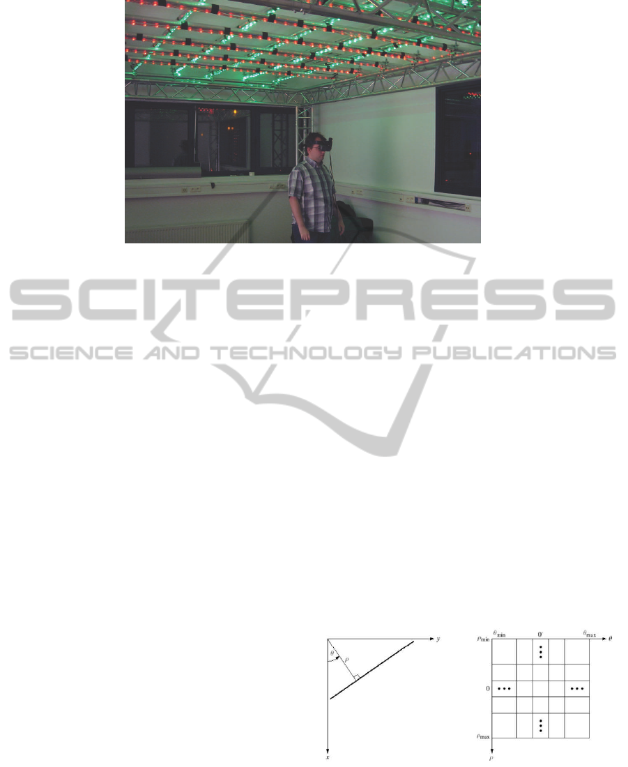
Figure 1: Our lab set-up with a 4 by 3 meter grid of LED ropes on the ceiling. The camera mounted on the virtual reality
glasses tracks its position and orientation by filming this grid.
3.2 Overview Algorithm
Our tracking algorithm gets the images of the camera
as input. The extrinsic parameters will be estimated
in the following steps:
• Detection of the LED ropes
• Calculating orientation from vanishing points
• Calculating position with known orientation
These steps will be explained in detail in the following
sections.
4 DETECTION OF THE LED
ROPES
Our first task is the detection of our constructed grid
in the input image. We first segment the individual
LEDs by evaluating the hue value of each pixel. Then
we use a simple ’flood fill’ algorithm to cluster the
pixels corresponding to a LED and retain only its cen-
ter. That way we speed up the line detection consid-
erably and eliminate a lot of random noise.
Secondly if we use a real camera, we need to take
lens distortion into account. The effects of lens dis-
tortion are clearly visible when using a lens with a
wide field of view. It causes straight lines to bend,
especially near the edges. This is something we want
to avoid at all costs. Therefore we calculate the dis-
tortion parameters beforehand with ’GML Toolbox’
(V.VezhnevetsandA.Velizhev, 2005) based on the im-
age processing library OpenCV (Bradski, 2000). Un-
like the undistortion function in OpenCV, we do not
want to undistort entire images because that would be
prohibitory slow. Instead we create a lookup table to
undistort individual LEDs very fast.
Last step in the detection of the LED ropes is the
line pattern recognition in the collection of detected
LEDs. A mature technique for line pattern recogni-
tion is the patented Hough Transform (Hough, 1962).
4.1 Hough Transformation
In general the Hough transformation is a mapping
of the input points to a curve in a dual parameter
space. The parameterization of the pattern (in this
case a line) determines the used parameter space and
the shape of the dual curves. The most common used
parameterization maps an input point (x
i
,y
i
) to a si-
nusoidal curve in the ρθ-plane with equation:
x
i
cosθ+ y
i
sinθ = ρ (1)
The geometrical interpretation of the parameters
(θ,ρ) is illustrated in figure 2.
Figure 2: Left: Geometrical interpretation of the (θ, ρ) pa-
rameterization of lines. Right: Subdividing the parameter
space into accumulator cells. (Image courtesy: (Gonzalez
and Woods, 2001)).
The Hough algorithm (Gonzalez and Woods,
2001) attains its computational attractiveness (O(N))
VISAPP 2011 - International Conference on Computer Vision Theory and Applications
540
by subdividing the parameter space into so-called ac-
cumulator cells (Figure 2). Each input point gener-
ates votes for every accumulator cell correspondingto
its mapped sinusoid in parameter space. Finally the
accumulator cells with the highest amount of votes
(most intersections) represent the line patterns in the
input space.
Although the Hough algorithm has a linear time
complexity, it has a high constant cost of ’drawing’
and searching for ’highlights’. Therefore most Hough
transformations cannot be performed in real-time. Al-
though we only have a small number of input points,
the high constant cost weighed heavily on the trackers
speed. Therefore we propose another line parameter-
ization to speed up the calculations with a relatively
small amount of input points.
4.2 Line Parameterization with Circles
To increase the speed and accuracy of the line de-
tection, we propose to calculate the intersections in
the Hough parameter space analytical. But this isn’t
trivial with sinusoidal curves (eq. 1). Therefore we
propose a new parameterization that maps each input
point (x
i
,y
i
) to a circle in the XY-plane with equation:
x−
x
i
+C
x
2
2
+
y−
y
i
+C
y
2
2
=
p
(x
i
−C
x
)
2
+ (y
i
−C
y
)
2
2
!
2
(2)
with (C
x
,C
y
) a fixed point in the image, like the prin-
cipal point. This means that for every point (x
i
,y
i
)
we will construct a circle with the midpoint between
(x
i
,y
i
) and (C
x
,C
y
) as center and radius equal to half
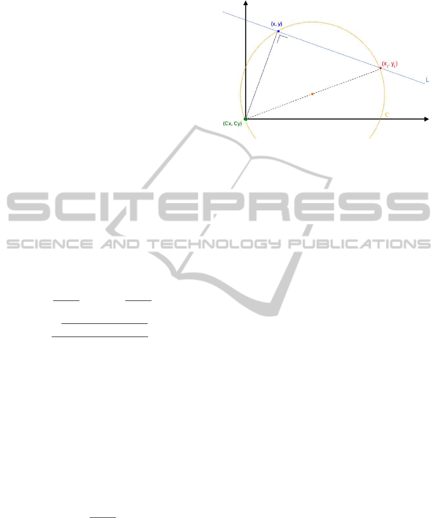
the distance between these two points. The geometri-
cal interpretation of this parameterization is shown in
Figure 3.
The analytic intersection point of 2 circles is much
easier to calculate than with 2 sinusoids. Given 2 cir-
cles with centers C
0
and C
1
and radiuses r
0
and r
1
and
the fixed point C, we can calculate the second inter-
section point P (first intersection point is C) as fol-
lows:
P = (C
0
+C
1
) +
r
2
0
− r
2
1
d
2
(C
1
−C
0
) −C
with d the distance between C
0
and C
1
.
In practice, we will represent each line with this in-
tersection point P. This ’line center’ defines a line
through this center P and perpendicular to the direc-
tion
~
PC.
Figure 3: Geometrical interpretation of the circle parame-
terization of lines. Each line L through input point (x
i
,y
i
) is
characterized by a point (x,y) ∈ C.
4.3 Line Detection with the New
Parameterization
To detect lines in our input image, we try to esti-
mate the most apparent line centers. For every LED
in the input image, we try to estimate a local direc-
tion/line, e.g. by using the closest LED. Each of these
lines defines a line center in the line parameterization
space. Noise and measurement errors cause the lo-
cal line centers representing the same line to slightly
vary their position. This means that we must define a
dynamic error bin around possible groups of line cen-
ters. The bins with the most points represent the most
apparent line patterns in the image. The algorithm has
an average complexity of O(N
2
). In applications with
a small set of input points -like our tracker- our Hough
algorithm greatly outperforms the standard algorithm.
5 CALCULATING ORIENTATION
FROM VANISHING POINTS
The lines detected in the previous step are the pro-
jections of the constructed parallel lines. Therefore
we know that each set of lines corresponding to one
axis (one color of LEDs) intersects in a single point,
the vanishing point. Classically the best fit intersec-
tion point of the lines is used as the vanishing point.
This can introduce a lot of jitter in the vanishing
point when the lines are nearly parallel. Therefore
we propose to calculate the vanishing direction sep-
arate from the distance to the vanishing point. The
vanishing direction is the direction from the principal
point of the camera to the 2D position of the vanish-
ing point. If we used the principal point as the fixed
point in the line detection step (§4.2), it can be shown
SCALABLE OPTICAL TRACKING - A Practical Low-cost Solution for Large Virtual Environments
541
that the vanishing direction D equals the interpolation
of two line directions D
1
and D
2
:
D = ||l
2
, pp|| ∗ D
1
+ ||l
1
, pp|| ∗ D
2
(3)
with pp the principal point and l
1
, l
2
the line cen-
ters from lines L
1
and L
2
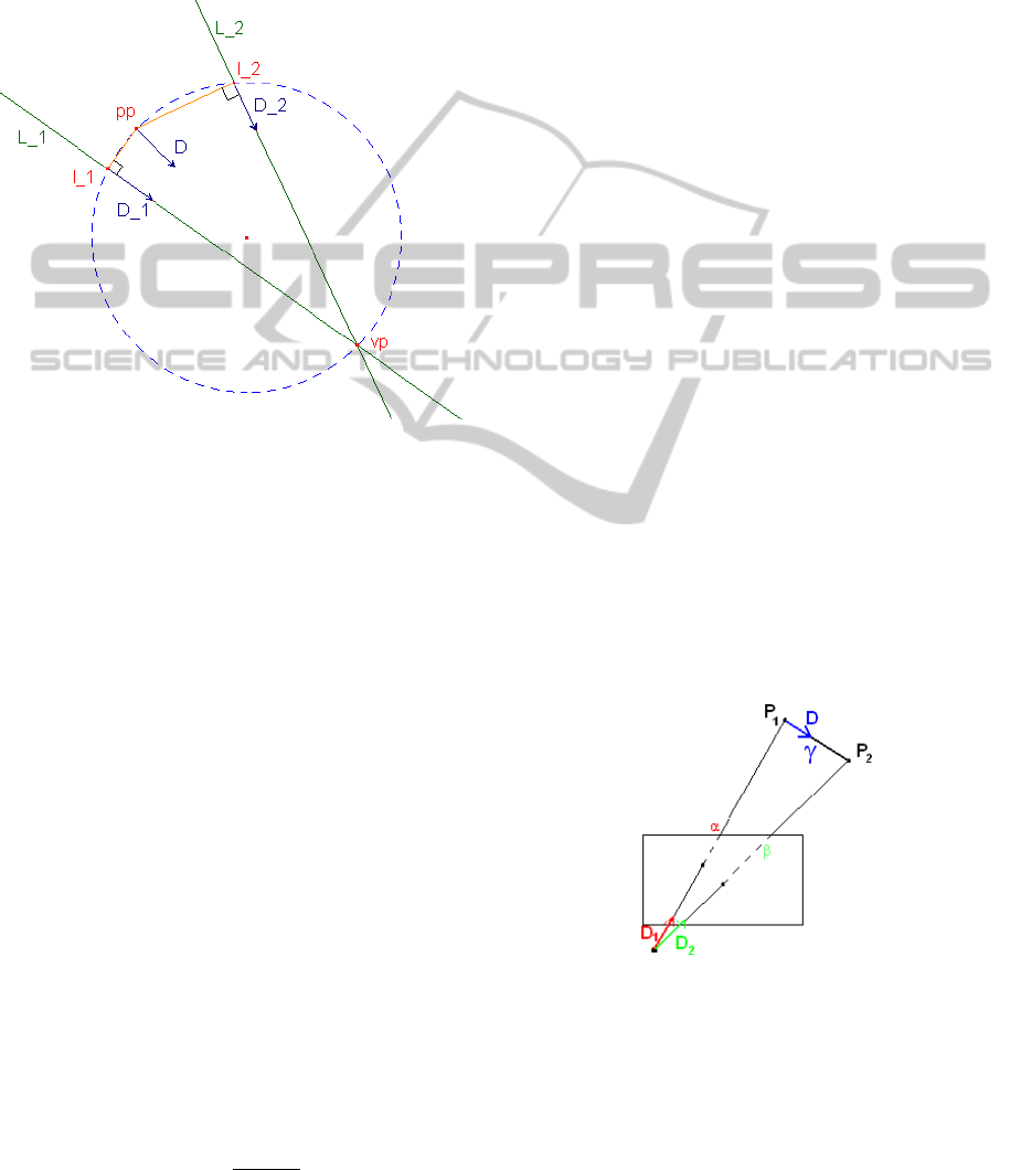
. Figure 4 gives a geomet-
ric representation of the interpolation. The vanishing
Figure 4: Calculating the vanishing direction D separate
from vanishing distance. The fixed point in this parameteri-
zation is the principal point pp. vp is the vanishing point of
lines L
1
and L
2
, with l
1
and l
2
as their line centers and D
1
and D
2
their line directions.
point corresponds with a point at infinity (intersec-
tion of parallel lines) and therefore is unaffected by
translation. This means that we can calculate the ro-
tation independent from the translation (Caprile and
Torre, 1990; Cipolla et al., 1999). We can see this
clearly in the projection equation of the vanishing
point V
i
= (u
i
,v
i
,w
i
), the projection of the point at in-
finity D
i
= (x
D,i
,y
D,i
,z
D,i
,0) (direction of the parallel
lines):
λ
i
u
i
v
i
w
i
= K[R|T]
x
D,i
y
D,i
z
D,i
0
(4)
with λ
i
a scale factor, K the calibration matrix with
the intrinsic parameters, R the rotation matrix and T
the translation vector. Which gives us:
λ
i
K
−1
V
i
= RD
i
(5)
The only unknown factor λ
i
can be calculated using
the fact that the inverse of a rotation matrix is its trans-
pose (so R
T
R = I) (Foley et al., 1996) and D
i
is a
normalized direction vector (so D
T
i
D
i
= 1):
λ
i
= ±
1
|K
−1
V
i
|
(6)
By using the coordinates of the found vanish-
ing points with their corresponding directions (X-,Y-
,Z-axis), the rotation matrix can be calculated from
Equation 5. Because of the uncertainties of the sign
of λ
i
, the orientation is ambiguous but this can be
solved by looking at previous frames or adding an ex-
tra marker.
The calculation of the 9 unknowns of the 3x3 ro-
tation matrix seems to require 3 vanishing points. But
knowing that the 3 rows of the matrix form an orthog-
onal base (Foley et al., 1996), we only need 2 corre-
spondences and therefore only 2 axis must be visible
at all times (in our case the X- and Y-axis, the ceiling).
6 CALCULATING POSITION
WITH KNOWN ORIENTATION
Given the rotation matrix and point or line correspon-
dences between frames, the direction of the transla-
tion can be recovered (Caprile and Torre, 1990). The
length of the translation is impossible to determine
without a reference distance in the input image. In
our system we choose to use the known interdistance
between LED ropes.
Caprile (Caprile and Torre, 1990) demonstrates
that by using 2 image points (with camera directions
~
D
1
and
~
D
2
) and known length γ and orientation
~
D be-
tween the world coordinates of points P
1
and P
2
, we
can calculate the distances to both points (α and β) by
triangulation (see Figure 5). Thus we have the follow-
ing system of linear equations with unknowns α and
β:
γ
~
D = β
~
D
2
− α
~
D
1
(7)
Figure 5: Depth estimation (α,β) of two points P
1
and P
2
can be done by a simple triangulation given the distance γ
and spatial orientation
~
D of the chosen points.
Given the rotation matrix calculated in the previ-
ous step, we undo the rotation on the lines. What we
get is a regular grid parallel to the image plane. Since
we know the distance between two neighboring lines,
the absolute distance to the ceiling can be calculated
VISAPP 2011 - International Conference on Computer Vision Theory and Applications
542
by using triangulation (Equation 7). It is also not re-
quired that the X- and Y-lines are at the same height, if
the distance between them is known. This fact makes
the construction of our lab set-up easier.
The only remaining unknown is the translation in
X- and Y- direction. Given the lines in the previous
frame, this translation can be trivially calculated.
7 RESULTS
The proposed algorithms have been implemented and
tested in a virtual set-up as well as in a real room-sized
lab set-up.
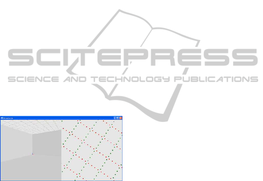
7.1 Virtual Set-up
To evaluate the soundness of our algorithm and de-
sign, we first constructed a virtual scene (see Figure
6). The virtual scene consists of a 8 by 10 meters
room and about 2.5 meters in height. The ceiling of
this room consists of a 2D grid of markers (LEDs) in
2 colors: red LEDs to indicate the lines parallel to the
X-axis and green to indicate those parallel to the Z-
axis. The distance between 2 adjacent parallel lines is
known, namely 50 cm.
Figure 6: Implementation of the virtual set-up. Left: view-
point of the user. Right: viewpoint of the tracker camera
and input of the tracking system.
A virtual test set-up has the advantage of knowing
the exact position and orientation of the user. We use
this data to evaluate our tracking system. The test con-
sists of a path through the virtual environment while
looking around. The run has been performed on a
standard pc and consists of about 400 frames at a res-
olution of 1024x768.
Figure 7(a) shows the calculated look- and up-
vectors defining the orientation of the camera poses
of the run. Because we have the real orientation of the
camera, we can calculate the absolute RMS error. We
find that the accuracy of our algorithm on relatively
noise free data is about 0.02
◦
for Yaw and 0.035
◦
for
Pitch and Roll.
Using this rotation, the path traveled by the cam-
era can be calculated (Figure 7(b)). We compare the
calculated positions with the real poses and get a RMS
accuracy of 4 millimeter in X- and Y-directions and
2.4 millimeter accuracy of the height of the camera.
Both orientation and position give a good result
under near optimal conditions. Therefore we built a
real set-up to test this under real-world conditions.
7.2 Lab Set-up
A virtual set-up is good to do the initial testing, but
our goal is off course to build a real tracking sys-
tem. So we constructed a room-sized (4x3 meter)
lab set-up as visible on Figure 1. Figure 9 shows
a input image of the camera that we want to track.
We use a ’Point Grey Flea Firewire’ camera captur-
ing 1024x768 images at 30 fps with a wide field of
view camera. Because we use LEDs, the shutter time
can be set at as little as 1 ms, which practically elim-
inates motion blur. This also implies that the system
can work in a large variety of lighting conditions, as
long as the LED’s are the brightest colored features.
Figure 8 shows the recording of estimated orientation
and position during a walk through our lab set-up.
Unlike the virtual set-up, we cannot compare the
results with absolute data. Therefore we captured
around 2000 frames at a stationary pose and took the
average as the ground truth position. The RMS er-
ror of the orientation tracker gives us an accuracy of
0.16
◦
Yaw and 0.23
◦
Pitch and Roll. The position
data gives us an accuracy of 5 millimeter in X- and
Y-direction and 8 millimeter in the Z-direction. If we
look at the processor time the camera tracker requires,
we see that it does not need more than 11 milliseconds
to compute. Most of this computing power (around
9.5 ms) is required to segment the LEDs, but still a lot
of processor power is left for other tasks or improve-
ments to our algorithm.
During tests, we’ve seen that the system func-
tions well under varying lighting conditions. How-
ever when used with the room lights, the LEDs under
the light can’t be segmented due to the camera’s low
dynamic range.
Although the tracking algorithm does not experi-
ence any drift, the global pose of persons using the
system can differ. Some sort of global starting posi-
tion must be defined if all participants need to be in
the same world space. There is also an inherit ambi-
guity in the global pose if the user moves when the
sensor is occluded. This problem could be improved
if we use an inertial sensor when line-of-sight is bro-
ken or by placing global positioning beacons.
SCALABLE OPTICAL TRACKING - A Practical Low-cost Solution for Large Virtual Environments
543
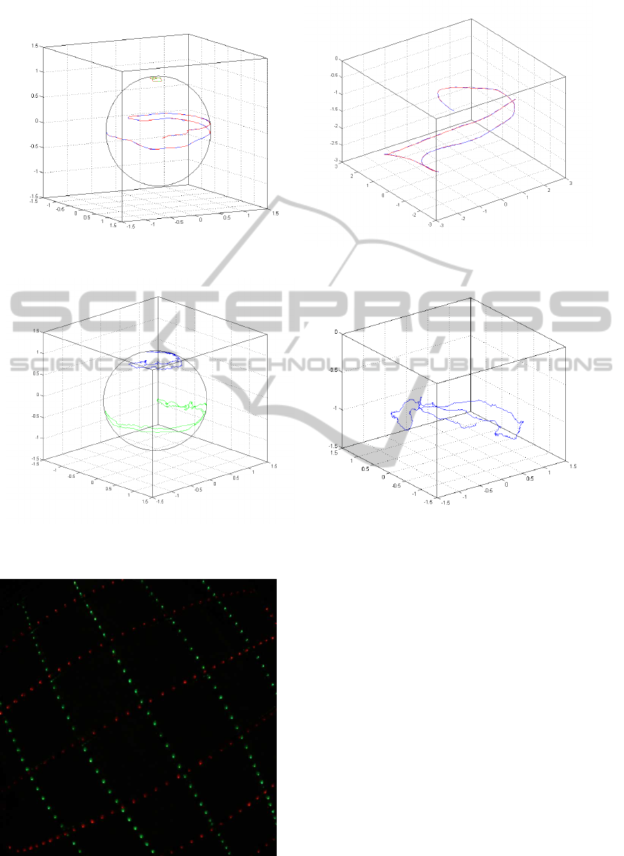
Figure 7: Results of the orientation and position tracker on input of a virtual camera. Left (a): Position of the look vector
(green) and up vector (blue) on the unit sphere with the original orientation overlaid (red). Right (b): Position of the camera
(blue) with the original position overlaid (red).
Figure 8: Tracking results of the camera tracker in a room-sized lab set-up. Left (a): Orientation of the calculated camera
with the look vector (blue) and up vector (green) on the unit sphere. Right (b): Estimated position of the camera in the lab.
Figure 9: Image from the camera in our lab set-up.
8 CONCLUSIONS AND FUTURE
WORK
In this paper we have proposed our low-cost wide-
area optical tracking system using regular cameras
and LED ropes. Our proposed real-time orientation
tracking algorithm using vanishing points has been
shown to be accurate and fast. This could be accom-
plished using a new parameterization of the Hough
transform for detecting line patterns. We are currently
looking at iterative refinement algorithms to get even
better results.
We are also looking to expand our current test set-
up to a larger theater room. This may require the
placement of global beacons to get an absolute po-
sition when line-of-sight is restored.
The first results from our tracking system are very
promising for a build-it-yourself wide-area tracker.
With orientation accuracy under 0.25 degrees and
VISAPP 2011 - International Conference on Computer Vision Theory and Applications
544

position errors smaller than 1 cm, our system can
compete with many expensivecommerciallyavailable
tracking systems on the market.
ACKNOWLEDGEMENTS
Part of the research at EDM is funded by the ERDF
(European Regional Development Fund) and the
Flemish government. Furthermore we would like to
thank our colleagues for their help and inspiration.
REFERENCES
Allen, B., Bishop, G., and Welch, G. (2001). Tracking:
Beyond 15 minutes of thought. In SIGGRAPH 2001,
Course 11.
Bishop, T. G. (1984). Self-tracker: a smart optical sensor
on silicon. PhD thesis, Chapel Hill, NC, USA.
Bradski, G. (2000). The OpenCV Library. In Dr. Dobbs
Journal of Software Tools.
Caprile, B. and Torre, V. (1990). Using vanishing points for
camera calibration. In Int. Journal Computer Vision.
Kluwer Academic Publishers.
Cipolla, R., Drummond, T., and Robertson, D. (1999).
Camera calibration from vanishing points in images
of architectural scenes. In BMVC ’99, British Machine
Vision Conference.
Foley, J. D., van Dam, A., Feiner, S. K., and Hughes, J. F.
(1996). Computer graphics: principles and practice
(2nd ed. in C). Addison-Wesley Longman Publishing
Co.
Foxlin, E. and Naimark, L. (2003). Vis-tracker: a wear-
able vision-inertial self-tracker. In IEEE Virtual Real-
ity 2003.
Gonzalez, R. C. and Woods, R. E. (2001). Digital Im-
age Processing. Addison-Wesley Longman Publish-
ing Co., New Jersey, 2nd edition.
Hough, P. V. C. (1962). Method and means for recognizing
complex patterns. United States Patent 3069654.
Raskar, R., Nii, H., Dedecker, B., Hashimoto, Y., Summet,
J., Moore, D., Zhao, Y., Westhues, J., Dietz, P., Barn-
well, J., Nayar, S., Inami, M., Bekaert, P., Noland, M.,
Branzoi, V., and Bruns, E. (2007). Prakash: lighting
aware motion capture using photosensing markers and
multiplexed illuminators. In SIGGRAPH ’07: ACM
SIGGRAPH 2007 papers, New York, NY, USA. ACM
Press.
Sutherland, I. E. (1968). A head-mounted three dimensional
display. In Proceedings of the 1968 Fall Joint Com-
puter Conference, AFIPS Conference Proceedings.
V.Vezhnevets and A.Velizhev (2005). Gml
c++ camera calibration toolbox.
http://research.graphicon.ru/calibration/gml-c++-
camera-calibration-toolbox.html.
Wang, J., Azuma, R., Bishop, G., Chi, V., Eyles, J., and
Fuchs, H. (1990). Tracking a head-mounted display
in a room-sized environment with head-mounted cam-
eras. In Proc. of Helmet-Mounted Displays II.
Ward, M., Azuma, R., Bennett, R., Gottschalk, S., and
Fuchs, H. (1992). A demonstrated optical tracker with
scalable work area for head-mounted display systems.
In SI3D ’92: Proceedings of the 1992 symposium on
Interactive 3D graphics. ACM Press.
Welch, G., Bishop, G., Vicci, L., Brumback, S., Keller, K.,
and Colucci, D. (2001). Highperformance wide-area
optical tracking: The hiball tracking system. In Pres-
ence: Teleoperators and Virtual Environments.
Welch, G. F. (1997). SCAAT: incremental tracking with in-
complete information. PhD thesis, Chapel Hill, NC,
USA.
Wormell, D., Foxlin, E., and Katzman, P. (2007). Advanced
inertial-optical tracking system for wide area mixed
and augmented reality systems. In EGVE 2007, 13th
Eurographics Workshop on Virtual Environments.
SCALABLE OPTICAL TRACKING - A Practical Low-cost Solution for Large Virtual Environments
545
