ILLUMINATING AND RENDERING HETEROGENEOUS
P
ARTICIPATING MEDIA IN REAL TIME USING
OPACITY PROPAGATION
Anthony Giroud and Venceslas Biri
University Paris Est, Marne-la-Vall´ee, LIGM, 77454 Marne-la-Vall´ee, France
Keywords:
Real-time rendering, Light scattering, Participating media, Propagation volume, Occlusion, Radial basis func-
tion.
Abstract:
We present a new approach to illuminate and render single scattering effects in heterogeneous participating
media in real time. The medium’s density is modeled as a sum of radial basis functions, and is then sampled
into a first volumetric grid. We then integrate the extinction function from each light source to each cell in
the volume by a fast cell-to-cell propagation process on the GPU, and store the result in a second volume. We
finally render both scattering medium and surfaces using a regular step ray-marching from the observer to the
nearest surface. As we traverse the medium, we fetch data from both volumes and approximate a solution to
the scattering equation. Our method is real-time, easy to implement and to integrate in a larger pipeline.
1 INTRODUCTION
Participating media are massively used nowadays,
both in applications where real-time is required, such
the video game industry and in interactive simula-
tions, as well as in domains where visual quality is
much more important than user interactions, like cin-
ema and animation.
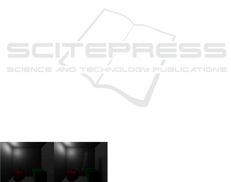
Figure 1: Left: the original scene. Right: a scattering media
i
s added.
Rendering natural phenomena such as clouds or
fog is absolutely not trivial, but is now compulsory
for any rendering engine, since these are the elements
in a scene which contribute the most to photorealism.
Considering the latest innovations and perfor-
mances of modern GPUs, it should be possible to illu-
minate and render heterogeneous fog or smoke more
easily and in real time.
Based on the three-steps algorithm and the
idea behind Light Propagation Volumes (Kaplanyan,
2009) where indirect radiance is propagated on sur-
faces, we introduce a new method to illuminate and
render in real time heterogeneous participating media
modeled as a sum of gaussians. We focus on single
scattering of light within an anisotropic medium, and
on shadow effects caused by the medium onto the ob-
jects. In this manuscript, we do not handle occlusions
by the geometry.
The contribution of this paper is:
• Establishing a modular framework to illuminate
and render inhomogenous scattering media.
• Introducing a new approach for the precomputa-
tion of the optical depth between each light source
and each point in the scene.
• Presenting an efficient implementation of this
framework.
2 PREVIOUS WORK
In this section, we only focus on single scattering
techniques. For more details about global illumi-
nation techniques, the reader is invited to refer to
(Cerezo et al., 2005). Scattering media rendering
techniques are classically divided in three categories:
analytic, stochastic and deterministic methods.
We focus on deterministic methods, that seek a
113
Giroud A. and Biri V..
ILLUMINATING AND RENDERING HETEROGENEOUS PARTICIPATING MEDIA IN REAL TIME USING OPACITY PROPAGATION.
DOI: 10.5220/0003374101130118
In Proceedings of the International Conference on Computer Graphics Theory and Applications (GRAPP-2011), pages 113-118
ISBN: 978-989-8425-45-4
Copyright
c
2011 SCITEPRESS (Science and Technology Publications, Lda.)

good approximation to media rendering equations
that can allow fast computation.
(Max, 1994) and (Nishita et al., 1987) worked on
an analytic solution for rendering atmospheric scat-
tering, one of the most studied applications by re-
cent works. Later, (Stam and Fiume, 1993) applied
Nishita’s model to render turbulent wind fields. More
recently, (Biri, 2006) presented an analytic reformu-
lation of the single scattering effect of a point light
source.
Using particles to model heterogeneous participat-
ing media appears much natural, and has also already
been intensively used (Stam, 1999; Fedkiw et al.,
2001).
(Zhou et al., 2007), propose an hybrid approach
to handle single scattering in an heterogeneous par-
ticipating medium, combining particles (i.e. gaus-
sians) and spherical harmonics. Despite good perfor-
mances, since all lighting computation depend on the
observer’s point of view, the whole pipeline has to be
processed at each frame. Moreover, it seems not con-
venient to implement and not easy to integrate in an
existing pipeline.
Approaches where the medium is discretized over
a 3D grid of voxels start with (Kajiya and Von Herzen,
1984). The scattering media is modeled as a set of
voxels of varying density. As a first step, the radiance
arriving at each voxel from each light source is com-
puted ; then, the main scattering integral is evaluated
iteratively between the viewer and the farthest voxel
intersected by a ray-tracing. Our method is inspired
from this two-step scheme.
(Kniss et al., 2003) present a technique to illu-
minate volumetric data based on half angle slicing
(Wilson et al., 1994), handling both a direct and an
approximated indirect lighting, but only for a single
light source situated outside the medium.
(Magnor et al., 2005) introduce a method to vi-
sualize reflection nebulae in interactive time. The
method uses a three-step algorithm similar to our
method, but where the medium’s density is kept un-
changed, due to the need for lighting precomputa-
tions.
Recently, (Kaplanyan, 2009) introduces the con-
cept of Light Propagation Volumes, to scatter indirect
lighting. After generating reflective shadow maps and
obtaining a set of virtual point lights on reflective sur-
faces, direct lighting is injected in a radiance volume,
which is a simple volumetric grid. In a third step,
using graphics hardware, indirect lighting is propa-
gated from cell-to-cell by iteratively solving differen-
tial schemes inside the volumetric grid.
Although focusing only on indirect lighting on
surfaces, this approach by propagation within a vol-
umetric grid is fast, allow more flexibility and could
as well be adapted in the case of direct incoming ra-
diance within a scattering media.
3 THEORETICAL BACKGROUND
3.1 Modeling the Participating Media
using a Radial Function Basis
Because our participating media is not static and can
evolve over time, the modeling step must be as simple
as possible for the user.
Like (Zhou et al., 2007), we choose to model our
heterogeneous participating media as a sum of radial
basis functions (RBF).
To define the medium’s appearance, the user just
provides a list of radial particles, which can differ in
both amplitude and scale. The particle’s density will
then be evaluated and injected into a 3D grid.
As the radial function itself, we simply chose the
gaussian function, defined on R
d
:
β(x) = ce
−a
2
kx−bk
2
(1)
where a ∈ R is its amplitude, b ∈ R
d
its center and
c ∈ R its scale.
To evaluate a function defined in a radial function
basis, we must sum all basis functions that overlay at
the given coordinates.
f(x) =
N
∑
i=0
β
i
(x) ⇐
⇒ f(x) =
N
∑
i=0
c
i
e
−a
2
i
kx−b
i
k
2
(2)
where i is the index of the RBF, and N is the total
number of RBFs in the basis.
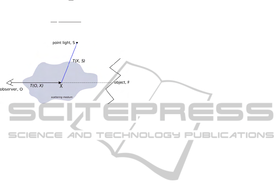
3.2 Our Illumination Model
The appearance of a participating medium is linked
to airlight (Arvo, 1993). When light is emitted from a
point light source S, then goes through a participating
medium which an extinction function f (see figure 2),
the light L
S
(O) received by the observer at position O,
who looks in the direction of point P is given by:
L
S
(O) =
Z
P
O
f(X)k(α(X))
I
S
kS− Xk
2
e
−T(O,X)−T(X,S)
dX
(3)
where k(α) is the scattering phase function, I
S
the in-
tensity of light S, and T(A, B) is the optical depth of
the medium between points A and B:
T(A, B) =
Z
B
A
K
t
(t)dt (4)
GRAPP 2011 - International Conference on Computer Graphics Theory and Applications
114
where K
t
is the extinction function of the medium.
In our method, we will assume an isotropic scat-
tering involving k(α(X)) =
1
4π
.
Therefore, our final model is:
L
S
(O) =
Z
P
O
f(X)
1
4π
I
S
kS− Xk
2
e
−T(O,X)−T(X,S)
dt
(5)
Figure 2: The integral of T(X, S) is computed during the
opacity propagation stage (blue path), between each light S
and each position X. The integral of T(O, X) is accumulated
at the rendering step.
4 OUR METHOD
4.1 Overview
Our pipeline is composed of three steps:
1. Density injection: The medium’s extinction func-
tion f is injected into a 3D grid, called the extinc-
tion volume (EV).
2. Opacity propagation: The optical depth T(S,X)
is integrated from each light source S to each cell
in another 3D grid called the opacity propagation
volume (OPV).
3. Volume rendering: The participating medium is
rendered, using a simple ray-marching technique,
and based on data obtained at the two previous
steps.
The following sections describe each step and de-
tail the algorithm. Our application is programmed us-
ing C++ and OpenGL, and GLSL for the shaders.
4.2 Density Injection
Since our medium is composed by a set of RBFs, the
final extinction coefficient at a given point within the
medium is obtained considering all particles that over-
lay at this point.
Thanks to the low frequency nature of the scatter-
ing medium, we can avoid such costly computation
on many points by pre-sampling the extinction coeffi-
cients on a 3D grid: the extinction volume.
The EV is implemented as a 3D texture, having
the same dimensions as the OPV. Each texel stores
only one decimal value, therefore a 16-bit floating
point encoding is sufficient. To fill the texture, we
perform a plane sweep along the Z-axis (depth). Each
plane sweep step fills one texture slice, which is
bound to a framebuffer object.
For each RBF contributing to the current slice, we
draw its bounding quad facing the camera. The RBF
is computed at each point on the quad using equation
2, evaluated in a fragment shader. Since several gaus-
sians may be overlayed on the same slice, we need to
activate additive blending.
4.3 Opacity Propagation
4.3.1 The Opacity Propagation Volume
Now that the medium’s density has been discretized
into voxels in the EV, we need to compute the optical
depth between each light source S and each EV cell X.
Contrarily to (Magnor et al., 2005), we allow both the
medium and lighting to evolve over time, and must
therefore consider repeating this step for each frame
for which these conditions have changed. To achieve
this in real time, our idea is to use the radiance gath-
ering scheme presented by (Kaplanyan, 2009) for in-
direct lighting on surfaces, and adapt it to propagate
(i.e. integrate) the optical depth between each light
source and each voxel in the EV. The resulting values
are stored in a separate grid: the opacity propagation
volume.
4.3.2 Propagation Scheme
When propagating radiance in a discrete neighbour-
ing, it is actually difficult to naturally simulate the
quadratic attenuation. When, like in (Kaplanyan,
2009), only cell-to-cell propagation directions are
considered, the radiance is distributed among all
neighbours and therefore scatters too rapidly around
the source, even in scenes without occluding surfaces
or media.
Because a scattering method is not adapted to an
implementation on graphics hardware, we instead use
a gathering scheme.
As each cell gathers optical depth from its six
neighbours and accounts for its own local density, our
solution is to consider both each discrete neighbour-
to-cell incoming directions and the accurate non-
discrete light-to-cell direction.
We compute a weighted mean of incoming optical
depth from all six neighbours, where the six weights
ILLUMINATING AND RENDERING HETEROGENEOUS PARTICIPATING MEDIA IN REAL TIME USING
OPACITY PROPAGATION
115
are determined by the similarity between the accurate
lighting direction
~
SX and the 6-connexity cell-to-cell
incoming direction, determined by their dot product.
As the light cannot arrive from a direction op-
posed to source, optical depth incoming with a neg-
ative scalar product must be discarded.
In other words, we have:
T
n+1
(X,S) = K(X) +
∑
5
i=0
W
S,i
(X)T
n
(X −
~
d
i
,S)
∑
5
i=0
W
S,i
(X)
(6)
where T
n
(X,S) is the portion of the density received
from source S by cell X at step n,
~
d
i
is the incoming
density direction from the i
th
neighbouring cell, and
which W
S,i
is the weight in the sum, given by:
W
S,i
= (1− K
t
(X))max
h
h
~
SX,
~
d
i
i,0
i
(7)
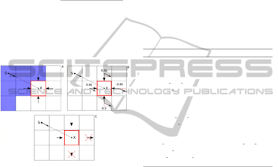
Figure 3: Optical depth gathering: weighting incoming di-
rections. A: Cells already visited by the propagation wave-
front are shown in blue, S is the position of the light source
and X is the center of the cell for which the gathering pro-
cess is detailed. B: We compute the dot product between
the non-discrete lighting direction
~
SX and each orthogonal
cell-to-cell direction. C: Neighbours whose dot product is
negative are discarded.
4.3.3 Algorithm
Like to the EV, the OPV is stored as a 3D 16-bit float-
ing point texture with the same dimensions. Each
texel stores one optical depth integral for each light
source, i.e. one texture is need per group of four
lights. Because using a texture for both reading and
writing in a shader is not available, the propagation
process which is implemented on the GPU requires
at least two copies of each texture. They are alterna-
tively used either for reading or writing at each new
step.
The integration originates from a single cell con-
taining the light, and advances radially like a wave-
front. By marking the visited texels using an addi-
tional texture, we can speed up the process in the
shader by discarding cells which either have already
been computed, or have not been reached yet.
To initialize a new propagation process, the two
OPV textures are cleared so that each texel starts with
zero, except for the cells which contain a light source,
which are initialized with their respectivelocal extinc-
tion coefficient.
Each single propagation step involves a plane
sweep along the texture slices. The gathering algo-
rithm is implemented in a fragment shader, called on
a fullscreen quad.
Algorithm 1 shows the pseudo-code of the frag-
ment shader for the gathering process.
Algorithm 1: Propagation - Pixel shader (GPU).
K(X) = Read local density from EV
for light source S do
/* 1. Gather density from neighbours */
wghtd dens sum = 0
weights sum = 0
for gathering direction
~
d
i
do
W
S,i
= max(dot(
~
SX,
~
d
i
), 0)
K(X −
~
d
i
) = Read neighbour density
wghtd dens sum += W
S,i
∗ K(X −
~
d
i
)
weights sum += W
S,i
end for
/* 2. Result for light S */
pxl
channels[S] = K(X) + wghtd dens sum /
weights sum
pixel color = pxl channels
end for
4.4 Rendering
4.4.1 Visualizing the Medium
Visualizing our participating medium means solving
the scattering equation 5, which defines how to obtain
the final color of each pixel.
Considering our model, we need to perform an in-
tegration along the view ray
~
OP. We have little choice
but solving this integration using a conventional ray-
marching over our grid.
We use a fixed integration step, even if more so-
phisticated techniques can be used (Giroud and Biri,
2010).
The entire algorithm is implemented on a frag-
ment shader, and is repeated separately for each light
source. We start the integration from the observer and
move in the direction of the surface in front of the
camera.
Based on precomputations performed in the two
GRAPP 2011 - International Conference on Computer Graphics Theory and Applications
116

previous sections, and considering equation 5, each
ray-marching step is straightforward:
1. Fetch f (X), the extinction coefficient correspond-
ing to the local density of our scattering medium,
and accumulate it with the values fetched at previ-
ous steps. At this point, the density of the medium
will decide how much light will locally not pass
through and thus be reflected, making the medium
visible to the camera.
2. Fetch T(X, S), the optical depth between X and
each separate light source S. The radiance from S
reaching X is obtained with: e
−T(X,S)
I
S
.
3. Compute quadratic attenuation: kS− Xk
−2
.
4. Compute this step’s contribution, and add the ra-
diance in the integral result:
L
S
(X) = (1− K
t
(X))L
S
(X) + K
t
L
IN
(X) (8)
where L
IN
(X) is the incoming radiance from the
source, given by:
L
IN
(X) = I
S
∗ e
−T(X,S)
(9)
5. Repeat until the nearest surface is reached.
4.4.2 Rendering Surfaces
Last but not least, in order to render the surface in
front of the current pixel, we have to use a simple
and fast illumination model. In our implementation,
we compute a simple Phong illumination, but other
models can be used as well.
The final pixel color is finally obtained as the re-
sult of an additional integration step, outside the main
ray-marching loop:
L
S
(O) = Ph
S
(P, O)e
−T(O,P)−T(P,S)
kS− Xk
−2
(10)
where Ph
S
(P, O) is the Phong illumination for light
S, at position P on the surface, and as perceived by
observer O.
5 RESULTS
This algorithm has been implemented using GLSL,
an Intel Core 2 Quad 2.8Ghz processor and a NVidia
GeForce GTX 280 graphics card. Screen resolution is
800x600.
Although classic ray-tracing based methods have to
perform again the major part of the computations at
each frame, our pipeline is very modular.
Which computation phases are or are not per-
formed at each new frame (see table 1) is the parame-
ter which impacts most on the speed at runtime.
Table 1: Depending on the type of scene, our method makes
it possible to precompute (P) the EV density injection and
the OPV propagation, and only update (U) volumes when
required.
Static elements Injection Propagation
Nothing U U
Medium P U
Lighting and medium P P
Table 2: FPS results with different volume resolutions and
lighting conditions. (P): phases 1 and 2 are precomputed.
Volumes size 1L(P) 1L 2L 4L 8L
15
3
320 62 62 51 34
20
3
251 38 37 35 22
30
3
203 17 17 16 9
40
3
120 9 9 9 5
In table 2, we can see that computing lighting for
between one and up to four sources does not bring
significant extra cost. With more than four lights, a
second OPV texture is required, which implies more
texture fetching and writing operations. In the second
column, only the rendering phase is performed.
Table 3: FPS results rendering mediums with different com-
plexities, with dynamic and static scenes, using extinction
and occlusion volumes with a 20
3
resolution, in our Cornell
box.
Nb RBFs Dynamic sc. Static sc.
1 38 251
125 36 250
1000 35 252
8000 22 215
27000 9 142
Table 3 shows that the medium’s dimensions al-
most only affect the density injection phase. After
phase 1, the complexity of the medium does not de-
pend on the number of particles anymore, but on the
number of cells in the extinction volume.
6 CONCLUSIONS AND FUTURE
WORK
In this paper, we presented a new method for illumi-
nating and rendering heterogeneous isotropic scatter-
ing media in real time. The medium is modeled by
providing a simple list of gaussians, which are first
sampled over a volumetric grid. Then, the optical
depth T(X, S) between each light source and each grid
cell is computed by propagating occlusions through-
out a second volume using a modified version of Cry-
ILLUMINATING AND RENDERING HETEROGENEOUS PARTICIPATING MEDIA IN REAL TIME USING
OPACITY PROPAGATION
117
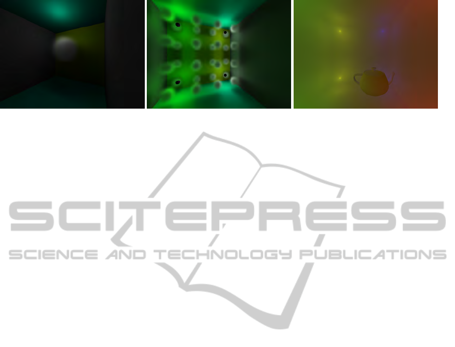
Figure 4: Left: Single large particle, one light. Middle: 16 particles, two lights. Right: Multiple lights in a thick fog.
tek’s algorithm. We finally render the medium and
surfaces by performing a ray-marching between the
camera and the nearest surface.
Our method fully achieves real time on conven-
tional hardware, and renders scattering effects such
as halos around light sources within the medium with
good quality. Using OpenGL and GLSL, we believe
that it is easy to implement and most of all, easy to
integrate in an existing graphics engine.
We are currently working at several improvements
to our method. First, by taking in account occlusions
by the geometry. Then, by optimizing the propaga-
tion algorithm so that the shader only processes cells
sutuated on the propagation wavefront. Finally, we
would like to speed-up our ray-marching, by optimiz-
ing GPU memory cache management.
REFERENCES
Arvo, J. (1993). Transfer equations in global illumination.
In Global Illumination, SIGGRAPH 93 Course Notes.
Biri, V. (2006). Real Time Single Scattering Effects. In Best
Paper of 9th International Conference on Computer
Games (CGAMES’06), pages 175 – 182.
Cerezo, E., Perez-Cazorla, F., Pueyo, X., Seron, F., and Sil-
lion, F. (2005). A survey on participating media ren-
dering techniques. the Visual Computer.
Fedkiw, R., Stam, J., and Jensen, H. W. (2001). Visual Sim-
ulation of Smoke. In proceedings of SIGGRAPH’01,
Computer Graphics, pages 15–22.
Giroud, A. and Biri, V. (2010). Modeling and Render-
ing Heterogeneous Fog in Real-Time Using B-Spline
Wavelets. In WSCG 2010.
Kajiya, T. and Von Herzen, B. P. (1984). Ray Tracing Vol-
ume Densities. In Computer Graphics (ACM SIG-
GRAPH ’84 Proceedings).
Kaplanyan, A. (2009). Advances in Real-Time Rendering
in 3D Graphics and Games Course. In SIGGRAPH
2009.
Kniss, J., Premoˇze, S., Hansen, C., Shirley, P., and McPher-
son, A. (2003). A model for volume lighting and mod-
eling. IEEE Transactions on Visualization and Com-
puter Graphics.
Magnor, M. A., Hildebrand, K., Lintu, A., and Hanson, A.J.
(2005). Reflection nebula visualization. IEEE Visual-
ization 2005.
Max, N. L. (1994). Efficient Light Propagation for Multiple
Anisotropic Volume Scattering. In proceedings of 5th
Eurographics Workshop on Rendering, pages 87–104.
Nishita, T., Miyawaki, Y., and Nakamae, E. (1987). A
Shading Model for Atmospheric Scattering consider-
ing Luminous Distribution of Light Sources. In pro-
ceedings of SIGGRAPH’87, Computer Graphics, vol-
ume 21(4), pages 303–310.
Stam, J. (1999). Stable Fluids. In proceedings of SIG-
GRAPH’99, Computer Graphics, pages 121–128.
Stam, J. and Fiume, E. (1993). Turbulent Wind Fields
For Gaseous Phenomena. In proceedings of SIG-
GRAPH’93, Computer Graphics, pages 369–376.
Wilson, O., Gelder, A. V., and Wilhelms, J. (1994). Direct
volume rendering via 3d textures. Tech. Rep. UCSC-
CRL-94-19.
Zhou, K., Hou, Q., Gong, M., Snyder, J., Guo, B., and
Shum, H.-Y. (2007). Fogshop: Real-time design and
rendering of inhomogeneous, single-scattering media.
In PG ’07: Proceedings of the 15th Pacific Confer-
ence on Computer Graphics and Applications, pages
116–125. IEEE Computer Society.
GRAPP 2011 - International Conference on Computer Graphics Theory and Applications
118
