
MORPHOLOGICAL ANTIALIASING AND TOPOLOGICAL
RECONSTRUCTION
Adrien Herubel, Venceslas Biri
LIGM, UPEMLV, Champs sur Marne, France
Stephane Deverly
Duran Duboi, Paris, France
Keywords:
Antialiasing, Mlaa, Topology, Realtime, Gpu.
Abstract:
Morphological antialiasing is a post-processing approach which does note require additional samples compu-
tation. This algorithm acts as a non-linear filter, ill-suited to massively parallel hardware architectures. We
redesigned the initial method using multiple passes with, in particular, a new approach to line length com-
putation. We also introduce in the method the notion of topological reconstruction to correct the weaknesses
of postprocessing antialiasing techniques. Our method runs as a pure post-process filter providing full-image
antialiasing at high framerates, competing with traditional MSAA.
1 INTRODUCTION
In computer graphics, rendering consists in sampling
the color of a virtual scene. The mathematical proper-
ties of the sampling operation imply that rendering is
inherently bond to aliasing artifacts. Therefore, the
subject of antialiasing techniques has been actively
explored for the past forty years (Catmull, 1978).
Traditional approaches to handle aliasing involve
computing multiple samples for each final sample.
However antialiasing by supersampling and its re-
finements for exemple MultiSamplge AntiAliasing
(MSAA), can be prohibitively costly notably in terms
of memory. Due to the popularity of deferred render-
ing approaches in recent real-time rendering engines,
a number of filter-based antialiasing techniques ap-
peared. Morphological Antialiasing (Reshetov, 2009)
(MLAA) is a relatively recent technique which en-
ables full image antialiasing as a post-process. Fig-
ure 1 compares two images corrected by respec-
tively MSAA and MLAA with similar results. How-
ever MLAA has its own caveats. As a pure image-
based techniques it can not handle subpixel geometry
aliasing. Moreover, as a non-linear filter, the tech-
nique uses proficiently deep branching and image-
wise knowledge thus is a poor candidate to a naive
GPU implementation.
We present in this paper both a practical real-
time implementation of the MLAA on the GPU and
a image-based technique to simulate subpixel geom-
etry antialiasing. Our GPU MLAA implementation
is a complete redesign of the original algorithm and
takes full advantage of hardware acceleration. We im-
prove results of MLAA on undersampled small scale
geometric details. Our algorithm is able to locally re-
construct subpixel missing data. Our method runs as a
pure post-process filter providing full-image antialias-
ing at high framerates.
2 ANTIALIASING TECHNIQUES
2.1 Supersampling
Antialiasing is a widely studied topic in computer
graphics from the very start (Catmull, 1978). An-
tialiasing is built in most graphics hardware (Akeley,
1993; Schilling, 1991) thanks to refinements of the
supersampling technique. In this technique, named
SSAA for Supersampling AntiAliasing, rendering is
done at higher resolution then undersampled to pro-
duce the final image. Though this technique gives
good results, it can be particularly costly in terms of
rasterization, shading and memory. Framerates can
decrease rapidly in case of complex shading or ray-
187
Herubel A., Biri V. and Deverly S..
MORPHOLOGICAL ANTIALIASING AND TOPOLOGICAL RECONSTRUCTION.
DOI: 10.5220/0003373201870192
In Proceedings of the International Conference on Computer Graphics Theory and Applications (GRAPP-2011), pages 187-192
ISBN: 978-989-8425-45-4
Copyright
c
2011 SCITEPRESS (Science and Technology Publications, Lda.)
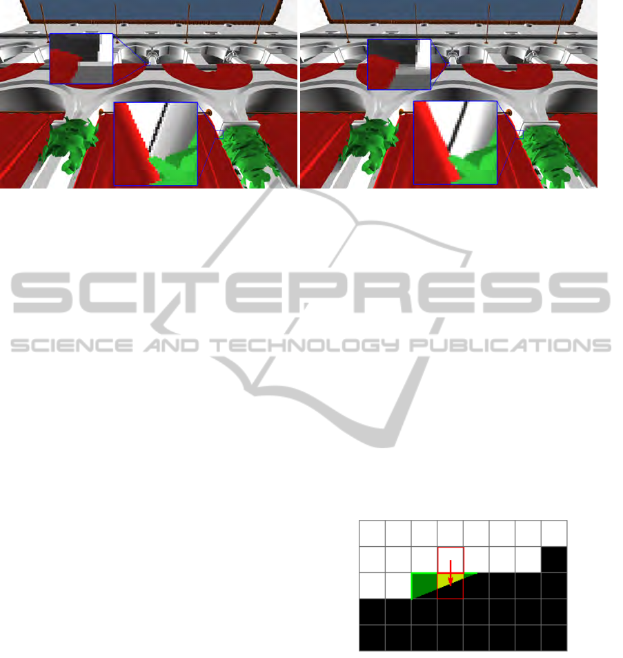
Figure 1: Left : Antialiasing with MSAA 4x. Right : with MLAA.
tracing.
The most common hardware supersampling ap-
proach is multisampling or MSAA (Akeley, 1993;
Schilling, 1991). In the naive supersampling, each
sample is shaded, therefore a pixel is shaded multi-
ple times. MSAA decreases the cost by decoupling
fragment shading and sampling. For each sample
in a pixel, the covering triangle is stored, shading is
then performed once for each covering triangle then
pixel color is extrapolated. CSAA or Coverage Sam-
pling Antialiasing reduces even more the number of
shaded samples by handling separately primitive cov-
erage, depth, stencil and color. Amortized Supersam-
pling (Yang et al., 2009) uses temporal coherence be-
tween frames to reduce computed samples but is lim-
ited to procedural shading.
Multisampling techniques are still tightly coupled
to fixed parts of the graphic pipeline, but fixed func-
tions tend to disappear. A recent technique by (Iour-
cha et al., 2009) takes advantage of new hardware
MSAA capabilities to acquire more accurate cover-
age values using neighbors of samples.
In deferred shading(Koone, 2007), the shading
stage is performed in image-space on G-Buffers.
Therefore using hardware multisampling with de-
ferred shading is usually considered challenging (En-
gel, 2009).
2.2 Image-based Antialiasing
In order to totally remove the dependency to geom-
etry, it is possible to directly filter the final image.
Full-image filtering offers the advantage of handling
triangle coverage aliasing as well as shadows or tex-
tures indifferently. With the recent gain in popularity
of deferred shading techniques and the limited MSAA
capabilities of the current generation of game console
these approaches flourished. The combination of edge
detection and blur is a common and inexpensive tech-
nique (Shishkovtsov, 2005), however the results con-
tain lots of false positive resulting generally in over-
blurring. In (Lau, 2003), 5x5 masks are used to de-
tects patterns to blend.
MLAA (Reshetov, 2009) is an image-based algo-
rithm providing full-image antialiasing independently
of the rendering pipeline. Therefore it can be used
in rasterization as well as in raytracing. Moreover it
is perfectly adapted to deferred rendering techniques.
The initial algorithm is CPU based and was success-
fully ported to SPU for the PS3 console (Hoffman,
2010) with results comparable to MSAA4x.
The algorithm can be coarsely divided in two
passes. First we detect discontinuity segments along
lines and columns of the image. Crossing segments
are then detected and form L shapes of varying ori-
entations and sizes. Then the pixels of the frame
Figure 2: In MLAA, the bottom red pixel blends with the
top red pixel weighted by the area of the yellow trapeze.
The technique consists in detecting L shapes in green and
blending pixels along the green triangle with pixels oppos-
ing the L.
are blended with their opposite neighbor along the-
ses shapes (cf. figure 2). Concerned samples are
those contained in the L, they are covered by a trapeze
which is a sub-part of the triangle formed by the L.
Blending weight depends of the trapeze area.
Though this algorithm is naively parallelizable it
is ill-suited to massively parallel architectures such as
GRAPP 2011 - International Conference on Computer Graphics Theory and Applications
188

GPU. Indeed L shapes detection imply deep dynamic
branching and quasi-random access patterns in the
frame which cripples cache efficiency (Nvidia, 2007).
Moreover, as a post-processing technique, MLAA is
unable to handle small scale geometry aliasing, and
as a relatively local filter can suffer from poor tem-
poral coherence, which induces flickering artifacts in
animation. Finally, using luminance for discontinuity
computation can lead to poor quality on RGB render-
ing.
3 MLAA ON THE GPU
3.1 Overview
The initial algorithm was entirely redesigned to fit
with a GPU GLSL implementation thus allowing di-
rect usage in any rendering engine. GPU detection
and storage of L shapes can be avoided since the
main objective is to compute the area of the covering
trapeze on each pixel along discontinuity lines. This
area can be computed using the pixel position on the
L shape. Our algorithm will therefore detect discon-
tinuity segments, determine relative positions of pix-
els along these segments, compute covering trapeze
areas and then do the final blending. The figure 3
shows an overview of the algorithm and samples for
each of these stages. Complete source code, including
shaders, can be found (Biri and Herubel, 2010).
discontinuity
detection
distance
propagation
blending map
computation
pixel
blending
Figure 3: Algorithm overview.
3.2 Discontinuities Detection
In this stage, we seek color discontinuities between
two neighboring pixels. For greyscale images, we de-
tect discontinuity presence if the difference between
greyscale values exceeds a user defined value called
the discontinuity factor, chosen between 0. and 1. For
color images we could use this factor as a threshold
in the luminance of the pixels. However in RGB, red
and blue share the same luminance leading to aliasing
artifacts on textures. Therefore we switch to CIELAB
color space where we are able to compute a color dif-
ference directly based on human perception (Kang,
2006). This discontinuity detection pass creates a tex-
ture containing, for each pixel, the existence of a dis-
continuity at its bottom and its right border. These
two booleans are stored in two different texture chan-
nels.
We also use this first stage to initialize the texture
storing discontinuity line lengths. We simply write 1
to the left and right distance of any pixel belonging to
horizontal lines and 1 to up and down distance to the
ones belonging to vertical lines. This is done simply
using MRT.
3.3 Distance Propagation
In this stage, we want to compute the distance in num-
ber of pixel, from any pixel along discontinuity lines
to their two extremities. In fact, we will propagate
distance from the extremities. This is done in left
and right direction for horizontal lines and on up and
down directions for vertical ones. Adding these two
lengths also gives us the total length of the horizontal
(resp vertical) discontinuity line minus one. And of
course, it gives us the position of the pixel relatively
to this line which will be useful in the next step. All
lengths will be computed in pixel distance.
To propagate the distance to the extremities of
lines, we will use a modification of the recursive dou-
bling approach (Dubois and Rodrigue, 1977; Hensley
et al., 2005). The computation will be done in up to
four steps. The first one will compute length distance
up to four pixels, the second one up to 16, the third
one up to 64 and the final one, up to 256. At each
step, for a given pixel X, we look at its distance d(X)
(for instance for left direction), fetch distance of the
texel at d(X) distance (at left) and add it to the current
distance d(X). Updating the distance is given by :
d(X) := d(X) + d(X.x − d(X).x,X.y) (1)
We do the same for right, up and down direction. We
also do that three times at each step. Figure 4 illus-
trates computation of left distance for the two first
steps of this stage. The reason we split the compu-
tation in several step is that, you can check, for each
step and pixel, if the pixel’s distance is below the max-
imum length we can obtain from the previous step. If
so, the pixel distance is already computed and can be
discarded.
Since distance will be stored in 8-bit precision, we
will restrict ourselves to 255 line length (in pixel).
The interest is that the four distance can be stored in
a regular RGBA texture. You need two such textures
in order to update distance, one texture for reading (in
the shader), and one for writing.
3.4 Computing Blending Factors
To this point we have computed the discontinuity seg-
ments, their lengths and the relative position of any
MORPHOLOGICAL ANTIALIASING AND TOPOLOGICAL RECONSTRUCTION
189
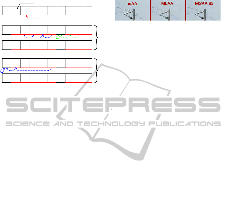
discontinuity line
0
1 1 1 1 1
initial distance value
0
1 1 1
0
1 1 1 1 1
0
1 1 1
0
1 2 3 4 4
0
1 2 3
S
T
E
P
1
0
1 2 3 4 5
0
1 2 3
0
1 2 3 4 4
0
1 2 3
A B
S
T
E
P
2
Figure 4: Overview of the recursive doubling approach to
compute the length of discontinuity lines. Example here
shows the computation of the relative distance to the left
horizontal end line. In the first step, pixel A checks its three
closest neighbor, each one making him “jump” to the left.
Pixel B checks its closest left neighbor then its left pixel
which does not belong to a discontinuity line (distance is
zero then). So the computation will add 0 for the two last
times. In the second step, pixel B has a distance lesser than
4, so it is discarded as all pixels marked in red. Pixel A will
check the fourth - its distance - left neighbor, add one, check
the left neighbor and stop here.
pixel along these lines. Therefore, for each pixel bor-
dering a discontinuity segment, we need to identify
which type of L shape it belongs to. Each pixel can
belong to up to four L shapes and will be blended ac-
cordingly. For an identified L shape, the area of the
trapeze A can be precomputed and depends from seg-
ment length L in pixels, and from the relative position
p of the pixel in the segment. Trapeze area can be
computed by the formula :
A =
1
2
1 −
2 ∗ p + 1
L
(2)
This equation is true if p < L/2, else we have a tri-
angle. If L is odd, the area of this triangle is 1/(2L),
else it is 1/(8L). Therefore, given the relative posi-
tion computed in previous step, and the length of the
L shape, we can fetch the blending factor in a precom-
puted 2D texture. Given that a pixel may belong to up
to for L shapes, four blending factors are stored, one
for each neighbor, on a RGBA texture which is used
in the final step.
3.5 Blending
At the end of the previous step, each pixel of the tex-
tures contains blending factors with its four neigh-
bors. Therefore the blending consists in using them
as local convolution kernels.
Figure 5: Comparison between no antialiasing (left),
MLAA (middle) and MSAA8x (right). Missing subpixel
data MLAA can’t close holes in the electrical lines.
4 TOPOLOGICAL
RECONSTRUCTION
An inherent problem to image based antialiasing algo-
rithm are their incapacity to “regenerate” geometry in
case of wrong sampling as in figure 5. We present in
this section a reconstruction technique for this geom-
etry, particularly in simple but frequent cases where
only one sample is missing. We use discrete geometry
and topology approaches to compute, for each pixel,
its connexity number (Kong and Rosenfeld, 1989) and
a characterization of its neighborhood. Using these
properties it is possible to determine whether a pixel
could reconnect two homogeneous areas and then “re-
construct” missing geometry.
4.1 Neighborhood and Connexity
In the case of binary images, we remind some el-
ements of digital topology (Kong and Rosenfeld,
1989). A point A ∈ Z
2
is defined as (A
1
,A
2
). We con-
sider neighborhood relationships N
4
and N
8
defined
by, for each point A ∈ Z
2
:
N
4
(A) =
B ∈ Z
2
; |B1 − A1| + |B2 −A2| ≤ 1
N
8
(A) =
B ∈ Z
2
; max(|B1 − A1|,|B2 − A2|) ≤ 1
(3)
Let α ∈ {4, 8}, we define N
∗
α
(A) =
N
α
(A)
A
. A point B
will be α-adjacent at point A if B ∈ N
∗
α
(A). An α-path
is a sequence of points A
0
...A
k
so that A
i
is adjacent
to A
i−1
for i = 1...k.
Let X ⊆ Z
2
, two points A,B of X are α-connected
in X if an α-path exists in X between these two points.
This defines an equivalence relation. Equivalency
classes for this relationship are α-connected compo-
nents of X. A subset X of Z
2
is said α-connected if it
is constituted by exactly one α-connected component.
The set constituted by all α-connected compo-
nents of X is noted C
α
(X). A subset Y of Z
2
is said
α-adjacent to a point A ∈ Z
2
if it exists a point B ∈ Y
adjacent to A. The set of α-connected components of
X α-adjacent to point A is noted C
A
α
(X). Formally, the
connexity number for a point A in a subset X of Z
2
are defined by :
T
α
(A,X) =
C
A
α
[N
∗
8
(A) ∩ X]
(4)
GRAPP 2011 - International Conference on Computer Graphics Theory and Applications
190
Using the number of connexities we can measure
efficiently the number of connected components adja-
cent to a given pixel.
4.2 Image Reconstruction
Our objective is to work on the particular case of a sin-
gle pixel missing for small scale geometry as shown in
Figure 6. In this case, post-processing techniques due
to missing data can not handle this artifact. Neverthe-
less, local image structure can indicate the probable
presence of a missing element.
We work locally on each image pixel on a 3x3
mask. On each mask we identify potential shapes
which are cut in two connected component by the
current pixel. We focus on pixels linking the two
connected components. The shape is constituted by
pixels sharing the same color and different from the
current pixel color. Reciprocally, the complement of
the reconstructed shape has to be a unique connected
component, thus sharing the same color as the current
pixel, in order to avoid removing straight lines. If X
is the shape to be reconstructed, we select pixels A so
T
8
(A,X) = 2 and T
8
(A,X) = 1. Therefore we can re-
place their color by the color of the shape. Figure 6
gives an overview of the results.
4.3 Integration
The correction takes place before discontinuity lines
detection. On the whole image, we compute the con-
nexity number for each pixel. In order to do this, we
compare the color in CIELAB space with its 8 neigh-
bors. Each neighbor with a different color than the
current pixel color is marked as belonging to X , the
others are marked as belonging to the set X. Using the
gathered data, the number of connexities is fetched
using a lookup-table. If the number of connexities
T
8
(A,X) = 2 and T
8
(A,X) = 1, the pixel is then re-
placed by the mean color of X pixels.
5 RESULTS
The algorithm was implemented on an Intel Core i7
920 with a NVidia GeForce GTX 295 graphic card.
Measurements were done on a Sponza-like scene at
resolution of 1920x1080. The Table 1 sums up the
results in terms of frames per second on our deferred
renderer. In this case MLAA performs well against
SSAA both in terms of quality and performance cost.
Note that our implementation is currently used on the
in-house real-time rendering engine at DuranDuboi
Studio notably for asset previewing.
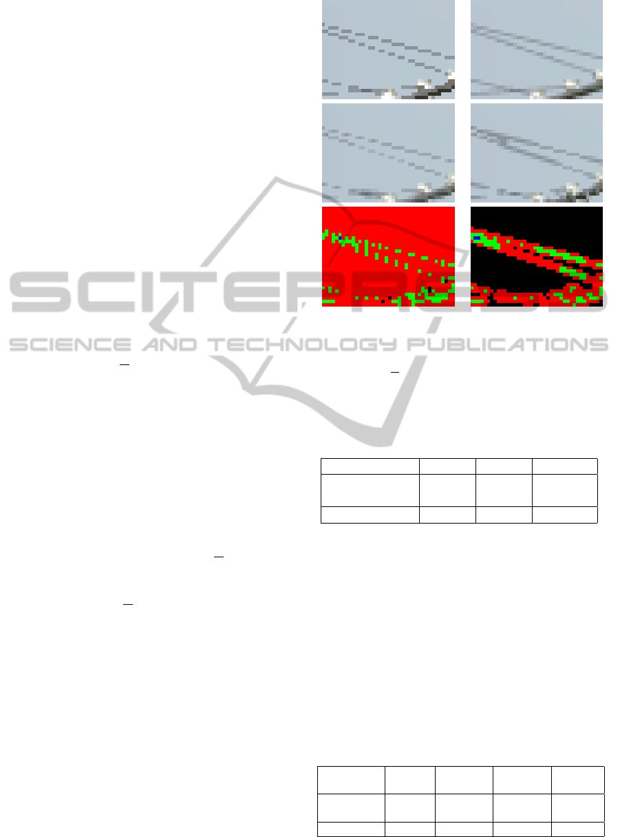
Figure 6: Detail of the reconstruction along electric lines.
Top left, original image. Top right, MSAA8x. Middle left,
MLAA without reconstruction. Middle right, MLAA with
topological reconstruction. Bottom line : connexity number
for X (left) and X (right), black = 0, red = 1, green = 2, other
> 2.
Table 1: FPS and additional cost of antialiasing techniques
on a deferred shading renderer.
Method No AA MLAA SSAAx2
Rendering 17.4 18.3 31.2
time (ms)
Add. cost (ms) 0 0.9 13.8
Figure 1 and table 2 compare antialiasing tech-
niques on a forward renderer. In terms of speed and
quality, MLAA is equivalent of MSAA4x.
However figure 5 illustrates a pathological case
for MLAA. Small scale geometry details lead to holes
between samples when the projected geometry is
smaller than pixel size. The topological reconstruc-
tion does have an additional cost of 0.55ms on our
testing configuration and prevent some of these arte-
facts. Figure 7 presents MLAA filtering with and
without correction on the whole image.
Table 2: FPS and additional costs of antialiasing methods
in a forward renderer.
Method no AA MSAA2 MSAA4 MLAA
Rendering
time (ms) 10.3 10.9 11.8 11.2
Add. cost 0 0.6 1.2 0.9
MORPHOLOGICAL ANTIALIASING AND TOPOLOGICAL RECONSTRUCTION
191
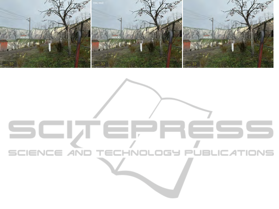
Figure 7: Original image (left), Standard MLAA (middle). MLAA with topological reconstruction (right).
6 CONCLUSIONS
In this paper, we presented a practical real-time im-
plementation of the MLAA algorithm suited to the
GPU. We introduced a new method using topological
reconstruction to handle pathological cases for image-
based antialiasing approaches. Our method improves
behavior of these algorithms on small scale geometric
details.
We intend to continue working on G-Buffer and
MLAA integration, particularly how to use additional
data in the G-Buffer such as depths and normals to
improve general MLAA behavior. We also aim to
improve the topological reconstruction to handle big-
ger gaps and to improve temporal coherence between
frames.
REFERENCES
Akeley, K. (1993). Reality engine graphics. In SIGGRAPH
’93: Proceedings of the 20th annual conference on
Computer graphics and interactive techniques, pages
109–116, New York, NY, USA. ACM.
Biri, V. and Herubel, A. (2010). Source code of TMLAA.
http://igm.univ-mlv.fr/ biri/mlaa-gpu/.
Catmull, E. (1978). A hidden-surface algorithm with anti-
aliasing. In Proceedings of the 5th annual con-
ference on Computer graphics and interactive tech-
niques, page 11. ACM.
Dubois, P. and Rodrigue, G. (1977). Analysis of the recur-
sive doubling algorithm. High Speed Computer and
Algorithm Organization, pages 299–305.
Engel, W. (2009). Deferred Shading with Multisampling
Anti-Aliasing in DirectX 10. in ShaderX7, W. Engel,
Ed. Charles River Media, March.
Hensley, J., Scheuermann, T., Coombe, G., Singh, M., and
Lastra, A. (2005). Fast summed-area table genera-
tion and its applications. Computer Graphics Forum,
24(3):547–555.
Hoffman, N. (2010). Morphological Antialiasing in God
of War III. http://www.realtimerendering.com/blog/
morphological-antialiasing-in-god-of-war-iii/.
Iourcha, K., Yang, J., and Pomianowski, A. (2009). A direc-
tionally adaptive edge anti-aliasing filter. In Proceed-
ings of the 1st ACM conference on High Performance
Graphics, pages 127–133. ACM.
Kang, H. (2006). Computational color technology. Society
of Photo Optical.
Kong, T. Y. and Rosenfeld, A. (1989). Digital topology: in-
troduction and survey. Comput. Vision Graph. Image
Process., 48(3):357–393.
Koone, R. (2007). Deferred Shading in Tabula Rasa, GPU
Gems 3, Nguyen, H.
Lau, R. (2003). An efficient low-cost antialiasing method
based on adaptive postfiltering. IEEE Transac-
tions on Circuits and Systems for Video Technology,
13(3):247–256.
Nvidia, C. (2007). Compute Unified Device Architecture
Programming Guide. NVIDIA: Santa Clara, CA.
Reshetov, A. (2009). Morphological antialiasing. In HPG
’09: Proceedings of the Conference on High Perfor-
mance Graphics 2009, pages 109–116, New York,
NY, USA. ACM.
Schilling, A. (1991). A new simple and efficient antialias-
ing with subpixel masks. ACM SIGGRAPH Computer
Graphics, 25(4):141.
Shishkovtsov, O. (2005). Deferred shading in stalker. GPU
Gems, 2 ch 9:143–166.
Yang, L., Nehab, D., Sander, P., Sitthi-amorn, P., Lawrence,
J., and Hoppe, H. (2009). Amortized supersampling.
In ACM SIGGRAPH Asia 2009 papers, pages 1–12.
ACM.
GRAPP 2011 - International Conference on Computer Graphics Theory and Applications
192
