
PARTICLE SMOOTHING FOR SOLVING AMBIGUITY PROBLEMS
IN ONE-SHOT STRUCTURED LIGHT SYSTEMS
F. van der Heijden, F. F. Berendsen, L. J. Spreeuwers and E. Schippers
Signals and Systems Group, Faculty of EEMCS, University of Twente, P.O.Box 217, 7500 AE Enschede, The Netherlands
Keywords:
3D Depth reconstruction, One-shot structured light system, Particle filtering, Jump Markov linear systems.
Abstract:
One-shot structured light systems for 3D depth reconstruction often use a periodic illumination pattern. Find-
ing corresponding points in the image and projector plane, needed for a triangulation, boils down to phase
estimation. The 2πN ambiguities in the phase cause ambiguities in the reconstructed depth. This paper solves
these ambiguities by constraining the solution space to scenes that only contain objects with flat surfaces, i.e.
polyhedrons. We develop a new particle filter that estimates the depth and solves the ambiguity problem. A
state model is proposed for piecewise continuous signals. This state model is worked out to find the optimal
proposal density of the particle filter. The approach is validated with a demonstration.
1 INTRODUCTION
We consider the problem of 3D object surface recon-
struction based on a sinusoidally modulated illumina-
tion pattern. Figure 1 shows an example. Depth infor-
mation of the surface is obtained from the phase of the
pattern observed by a camera. This is the principle of
phase-measuring profilometry (Su and Chen, 2001).
Sinusoidal patterns are beneficial because the phase
can be estimated easily and accurately, provided that
the period of the signal is small. This all can be done
with a single shot of the scene, thus allowing moving
objects. Since the phase of a sine has an ambiguity of
multiples of 2π, the depth derived from the phase is
also ambiguous. If the range of depths is limited to a
2π-zone, or if the depth is a smooth function without
jumps, the ambiguity is easily bypassed. Otherwise,
more involved methods must be applied. For that, two
principles are available. One possibility is to augment
the pattern such that more information becomes avail-
able (Su and Chen, 2001). The other possibility is to
constrain the solution space. In this paper we focus
on this second possibility. We only consider objects,
that are made up by flat surfaces, i.e. polyhedrons.
Amongst all possible solutions we have to select the
one that describes flat surfaces. With a suitable geo-
metrical set-up of the camera and the projector, this
particular solution can be made unique (van der Hei-
jden et al., 2009).
The question is how to find this unique solution.
We address this problem by scanning the image in
Figure 1: Sinusoidal illumination.
the phase direction along rows in the camera plane.
We use the row co-ordinate, denoted by ξ, as the run-
ning variable. Each row of the image is a mapping
from a 2D slice [X(ξ) Y (ξ) Z(ξ)] of the 3D surface
of the scene. Suppose that we have found the depth
co-ordinate Z(ξ). Then, using the pinhole geometry
of the camera, it is easy to find X (ξ) and Y (ξ). So,
we only need to concentrate on finding Z(ξ). For
simplicity, and without loss of generality, we ignore
the Y -co-ordinate, so that we have a 2D geometry, i.e.
[X(ξ) Z(ξ)].
Since the scene is made up by multiple objects,
the depth Z(ξ) contains step transitions. Between two
successive transitions, [X(ξ) Z(ξ)] form a linear seg-
ment due to the assumption of having flat surfaces.
Each linear segment can be represented by two pa-
rameters, e.g. the slope and the interception of the
depth. We model this piecewise linear behavior of
the depth with a system state equation for Z(ξ). The
state equation does not contain process noise except
for the step transitions that occur randomly. We esti-
mate the positions of the transitions as well as the two
parameters of each segment with a new particle filter.
531
van der Heijden F., F. Berendsen F., J. Spreeuwers L. and Schippers E..
PARTICLE SMOOTHING FOR SOLVING AMBIGUITY PROBLEMS IN ONE-SHOT STRUCTURED LIGHT SYSTEMS.
DOI: 10.5220/0003370005310537
In Proceedings of the International Conference on Computer Vision Theory and Applications (VISAPP-2011), pages 531-537
ISBN: 978-989-8425-47-8
Copyright
c
2011 SCITEPRESS (Science and Technology Publications, Lda.)
The input of the filter is formed by the sequence of
observed image intensities.
This is a fully different approach than the one pre-
sented in (van der Heijden et al., 2009). There, the
solution is expressed in terms of the instantaneous
frequency and its derivative, i.e. the first and sec-
ond derivative of the phase. Unfortunately, solutions
based on derivatives are often quite sensitive to noise.
The goal of this paper is to provide a first proof of
principle. We will demonstrate that particle filtering
is a feasible solution to the problem. The original-
ity of the paper is that we show that particle filtering
is able to unambiguously estimate this class of piece-
wise linear signals even though the measurements are
ambiguous. Section 2 introduces the geometrical set-
up. The model and the particle filter are described in
Section 3 and 4. The filter is validated with a demon-
stration in Section 6.
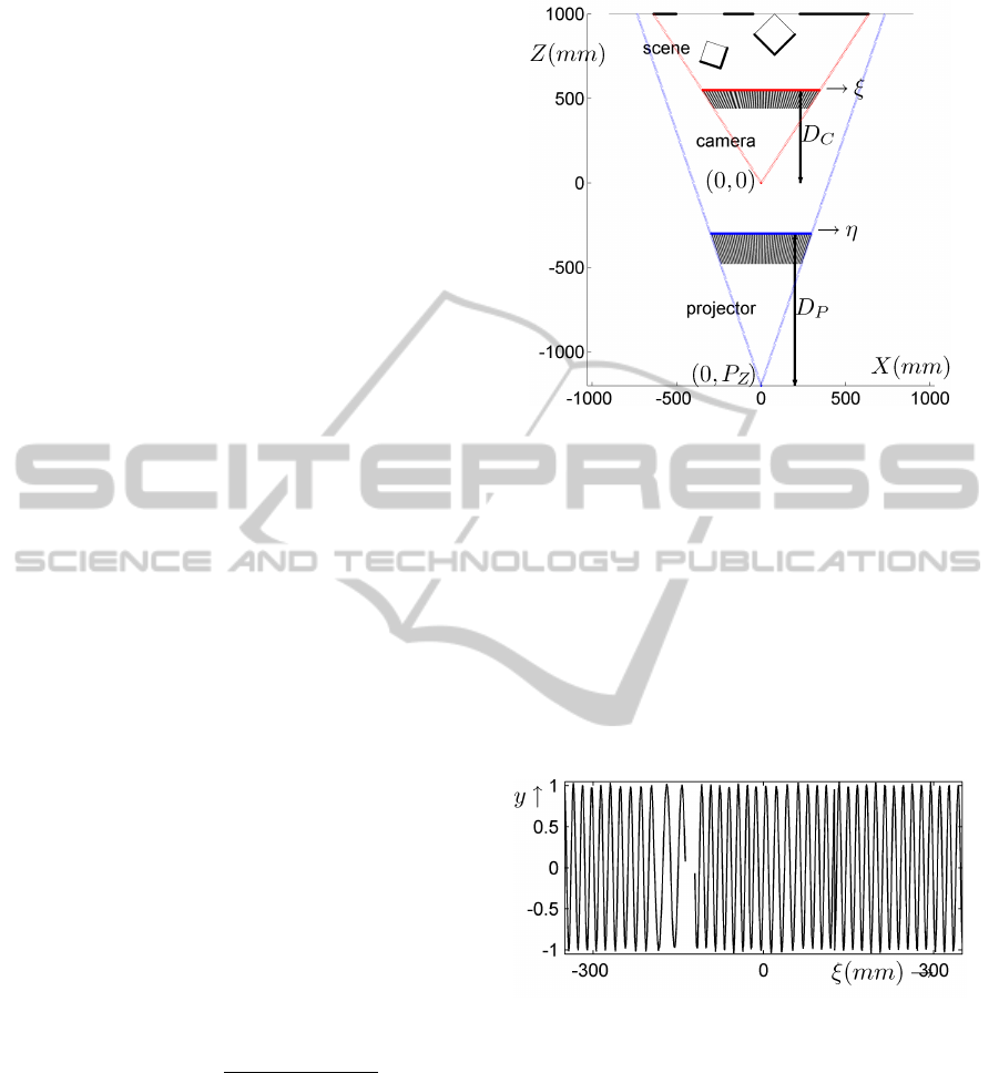
2 SCENE, CAMERA AND
PROJECTOR GEOMETRY
For simplicity, we choose a camera/projector geome-
try such that the projector is placed exactly behind the
camera. Other configurations are also possible, but
the mathematics becomes more involved then. Figure
2 gives the geometry for the 2D case, i.e. for one scan
line. The camera center is located at the origin. The
projector center is at (0, P
Z
). Both devices have their
optical axes pointing in the Z-direction. The focal dis-
tances of the camera and the projector are D
C
and D
P
.
We assume that the projector emits rays according to
a pattern Asin(2πη/T ) where η is the running vari-
able in the projector plane, and T is the period of the
pattern.
The measurement function h(Z,ξ) follows from
the pinhole equations XD
P
= (Z − P
Z
)η and
XD
C
= Z ξ of the projector and the camera:
h(Z(ξ), ξ) = B sin
2π D
p
Z(ξ) ξ
D
C
T (Z(ξ) − P
Z
)
(1)
The amplitude B is assumed to be constant. In prac-
tice, B depends on the radiometric properties and the
geometry of the objects and the illumination. There-
fore, in a real application, B will slowly variate with
ξ. This complicates the problem since we will need
to augment the state vector to embed the variation of
B in the state model. On the other hand, it may also
facilitate the estimation since step edges in B(ξ) is a
clue for discontinuities in the depth Z(ξ). As our goal
is only to provide a first proof of principle we ignore
the possible variation of B.
Figure 2: Camera and projector geometry.
The measurements y
k
are obtained by uniform
sampling along ξ defining samples Z
k
= Z(ξ
k
) at
equidistant positions ξ
k
along the image plane:
y
k
= h
k
(Z
k
) + v
k
(2)
Here, h
k
(Z
k
) = h(Z
k
,ξ
k
), and v
k
is the measurement
noise. We assume uncorrelated Gaussian noise with
standard deviation σ
v
. Figure 3 shows the measure-
ments that correspond to the set-up in Figure 2. Note
that some intervals of ξ may lack data. This is because
of occlusion.
Figure 3: Measurements from the set-up of figure 2.
The likelihood function becomes:
p(y
k
|Z
1:k
) = p(y
k
|Z
k
) = N(y
k
,h
k
(Z
k
),σ
2
v
) (3)
The ambiguity of the measurement function is de-
picted in figure 4. Here, we show p(y
k
|Z
k
) for the
configuration and measurements in figure 2 and 3
as an intensity plot in the Z, ξ domain. The plot is
also given in the Z,X domain by application of a
geometric transform based on the pinhole equation
X = (Z ξ)/D
C
. The figures show various trajecto-
ries that are all compatible with the measurements.
The reddish thick lines are all solutions with ambigu-
ities that are due to the identity sin(φ) = sin(φ+ 2nπ),
VISAPP 2011 - International Conference on Computer Vision Theory and Applications
532
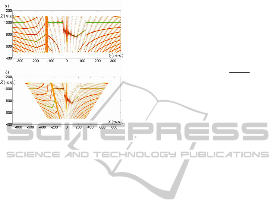
Figure 4: Ambiguous solutions in a) the Z, ξ domain, and b)
in the Z, X domain. The green lines form the ground truth.
whereas the thin almost vertical solutions are due to
sin(φ) = sin(π − φ + 2nπ). The green lines in the fig-
ures are the ground truth. The various trajectories in
the X,Z domain are all slightly curved, except for one:
the true solution. We also note in figure 4 that the am-
biguity near the optical axis of the projector dimin-
ishes. This is at the cost of an increasing noise sensi-
tivity. The figure also shows a cone where all X, Z are
evenly likely. This area corresponds to a part in the
scene that is not illuminated because of occlusion.
3 MODELING THE SYSTEM
Starting with the definition of the state vector, this
section introduces a suitable state equation. The state
vector that we consider consists of two continuous
states Z
k
,a
k
, and one Boolean state r
k
. Here Z
k
is
the depth at a position ξ
k
, and a
k
is the slope of the
surface, i.e. a
k
= ∂Z
k
/∂X
k
. We combine Z
k
and a
k
in
a 2D vector: x
k
= [Z
k
a
k
]
T
. The variable r
k
indicates
that a jump transition has taken place at position k.
The two possible outcomes are J and S , i.e. ”jump”
and ”smooth”, respectively. The probability of a jump
equals P
J
. We assume that the variable r
k
is memory-
less. That is: Pr(r
k
|r
0:k−1
,x
0:k−1
) = Pr(r
k
). If r
k
= J,
the vector x
k
is reset to a new, random state, drawn
from a bivariate uniform distribution:
p(x
k
|r
k
= J,r
0:k−1
,x
0:k−1
) = p(x
k
|r
k
= J)
= U (Z
k
,I
Z
)U (a
k
,I
a
)
(4)
U (Z
k
,I
Z
) denotes a uniform distribution of Z
k
within
an interval I
Z
.
If no jump takes place, i.e. r
k
= S, then x
k
pro-
ceeds continuously. From the pinhole equation X =
Zξ/D
C
and the definition of the slope a
k
= ∂Z/∂X it
is easy to derive that ∂Z/∂ξ = aZ/(D
C
− aξ). From
this, we obtain the following nonlinear system state
equation f
k
(x
k
):
x
k+1
=
Z
k+1
a
k+1
= f
k
(x
k
) =
"
Z
k
D
C
−aξ
k
D
C
−aξ
k+1
a
k
#
(5)
Since there is no process noise:
p(x
k
|r
k
= S,r
0:k−1
,x
0:k−1
) = δ(x
k
− f
k
(x
k−1
)) (6)
Within a continuity interval, x
k
proceeds determinis-
tically. Estimation of this part of a trajectory boils
down to estimation of two parameters, e.g. the in-
terception and the slope. Recurrent estimation of
these parameters can easily be accomplished by an
extended Kalman filter, provided that no jumps occur,
and that the measurements are unambiguous. These
two conditions are not met in the present case.
4 THE PARTICLE FILTER
Our approach is inspired on algorithms for jump
Markov linear systems as proposed in (Doucet et al.,
2001). The most important difference between the
model, discussed there, is that, conditioned on r
1:k
,
their system is Gaussian-linear, whereas our system
is not. If in (Doucet et al., 2001) the sequence r
1:k
is given, the corresponding sequence x
1:k
is Gaussian.
In our case, it is still multimodal. Especially, when a
jump occurs, x
k
is first uniform instead of Gaussian,
and after one measurement it becomes multi-modal.
We are able to solve the ambiguity because, after a
jump, the correct trajectory is constraint.
We adapted the algorithm in (Doucet et al., 2001)
as follows. We augment each particle r
(i)
1:k
by two
statistics: m
(i)
k|k
and P
(i)
k|k
. These are the posterior mean
of x
k
and the corresponding error covariance matrix,
respectively. The connotation is as follows. Suppose
that the last jump in the sequence r
(i)
0:k
has taken place
at position k
j
< k. At that position, a new sample x
(i)
k
j
is drawn from U (Z
k
,I
Z
)U (a
k
,I
a
). From that point on,
x
(i)
k
proceeds without jumps. Therefore, we can esti-
mate x
k
using an extended Kalman filter yielding the
statistics m
(i)
k|k
and P
(i)
k|k
.
We only need to work out the proposal den-
sity and the weight function to establish the al-
PARTICLE SMOOTHING FOR SOLVING AMBIGUITY PROBLEMS IN ONE-SHOT STRUCTURED LIGHT
SYSTEMS
533

gorithm. The optimal proposal density (Arulam-
palam et al., 2002) and (Doucet et al., 2001), is
p(r
k
,x
k
|r
(i)
0:k−1
,x
(i)
0:k−1
,y
k
). This is the density from
which we draw new samples. We write:
p(r
k
,x
k
|r
(i)
0:k−1
,x
(i)
0:k−1
,y
k
) =
p(x
k
|r
k
,x
(i)
0:k−1
,y
k
)Pr(r
k
|x
(i)
0:k−1
,y
k
) (7)
This shows that we first can draw a sample of r
k
, and
conditioned on that, a sample for x
k
. We concentrate
on r
k
first.
The first step is to expand Pr(r
k
|x
(i)
0:k−1
,y
k
) using
Bayes’ theorem:
Pr(r
k
= J|x
(i)
0:k−1
,y
k
) = (8)
P
J
p(y
k
|r
k
= J,x
(i)
k−1
)
(1 − P
j
) p(y
k
|r
k
= S,x
(i)
k−1
) + P
J
p(y
k
|r
k
= J,x
(i)
k−1
)
The density with r
k
= J in this expression follows
from eq. 3 and 4:
p(y
k
|r
k
= J,x
(i)
k−1
) = p(y
k
|r
k
= J) (9)
=
Z
+∞
−∞
p(y
k
,Z
k
) dZ
k
=
Z
+∞
−∞
p(Z
k
|y
k
) p(Z
k
) dZ
k
=
Z
+∞
−∞
N(y
k
,h
k
(Z
k
),σ
2
v
) U(Z
k
,I
Z
) dZ
k
The density in eq. 8 with r
k
= S follows from eq. 3
and 6:
p(y
k
|r
k
= S,x
(i)
k−1
) = N(y
k
,h
k
(f
k
(x
(i)
k−1
)),σ
2
v
) (10)
Substitution of eq. 9 and 10 in eq. 8 yields:
Pr(r
k
= J|x
(i)
0:k−1
,y
k
) = (11)
1 +
(1 − P
J
) N(y
k
,h
k
(f
k
(x
(i)
k−1
)),σ
2
v
)
P
J
R
+∞
−∞
N(y
k
,h
k
(Z
k
),σ
2
v
) U(Z
k
,I
Z
) dZ
k
!
−1
The result is quite intuitive. The fraction contains the
likelihood ratio under the two hypotheses r
k
= S and
r
k
= J, respectively. If the likelihood ratio is one,
the posterior probability equals the prior probability.
If the observed measurement matches the predicted
measurement, the likelihood ratio will be greater than
one, and as a result the posterior probability of a tran-
sition decreases.
Once a sample of r
k
has been drawn, we concen-
trate on x
k
. If we have drawn r
(i)
k
= J, the particle
jumps, and x
(i)
k
must be reset to a new, random state.
The distribution to drawn from is:
p(x
k
|r
k
= J,x
(i)
0:k−1
,y
k
) = (12)
1
k
C
k
N(y
k
,h
k
(Z
k
),σ
2
v
) U(Z
k
,I
Z
) U(a
k
,I
a
)
k
C
k
is a normalizing constant. The sample is the start
of a new smooth trajectory. We initiate the statistics of
that trajectory to m
k|k
= x
(i)
k
, and P
k|k
= diag(σ
2
Z
, σ
2
a
).
We set σ
2
Z
= σ
2
v
/H
2
(Z
(i)
k
) with H( ) the derivative of
h
k
(Z
k
). The variance of a
k
is set to 16 which covers a
wide band of slopes.
If we have drawn r
(i)
k
= S, the density
p(x
k
|r
k
= S,x
(i)
0:k−1
,y
k
) follows from an extended
Kalman update:
m
(i)
k|k−1
= f
k
(m
(i)
k−1|k−1
)
S = H
i
F
i
P
(i)
k−1|k−1
F
T
i
H
i
+ σ
2
v
K = F
i
P
(i)
k−1|k−1
F
T
i
H
i
S
−1
(13)
m
(i)
k|k
= m
(i)
k|k−1
+ K (y
k
− h
k
(m
(i)
k|k−1
))
P
(i)
k|k
= F
i
P
(i)
k−1|k−1
F
T
i
− K S K
T
F
i
is the Jacobian matrix of f
k−1
( ) evaluated at
m
(i)
k−1|k−1
. H
i
is the derivative of h
k
( ) at m
(i)
k|k−1
.
Beside a proposal density to draw samples from,
we also need a function to weight these samples. The
weight function that corresponds to the optimal pro-
posal density is w
i
k
= p(y
k
|x
(i)
k−1
). See (Arulampalam
et al., 2002).
w
i
k
=
∑
r
k
Z
+∞
−∞
p(y
k
|x
k
) p(x
k
|r
k
,x
(i)
k−1
) Pr(r
k
) dx
k
= P
J
Z
+∞
−∞
N(y
k
,h
k
(Z
k
),σ
2
v
) U(Z
k
,I
Z
) dZ
k
+ (1 − P
J
) N(y
k
,h
k
(f
k
(x
(i)
k−1
)),σ
2
v
) (14)
This equation works out differently for samples with
a jump and samples without. If the jump samples are
enumerated by i
J
and the other by i
S
, we find:
w
i
J
k
= P
J
Z
+∞
−∞
N
y
k
,h
k
(Z
k
),σ
2
v
U(Z
k
,I
Z
) dZ
k
w
i
S
k
= (1 − P
J
) N
y
k
,h
k
(m
(i
S
)
k|k
,σ
2
v
(15)
A cycle of the particle filter follows the following
code:
For the whole sample set i = 1, ··· , N:
• Sample r
(i)
k
from the distribution given in eq. 11.
• If r
(i)
k
is a jump: sample x
(i
J
)
k
from the distribution
given in eq.12. Initiate m
(i
J
)
k|k
and P
(i
J
)
k|k
accordingly.
VISAPP 2011 - International Conference on Computer Vision Theory and Applications
534
• If r
(i)
k
is smooth: update m
(i
S
)
k|k
and P
(i
S
)
k|k
. See eq
13.
• Evaluate the weights w
i
k
according to eq. 15.
• Normalize the weights w
i
k
←− w
i
k
/
∑
i
(w
i
k
).
• Resample to obtain unweighed particles.
The set
n
r
(i)
k
,m
(i)
k|k
o
, i = 1,2, ... provides us with a
particle estimate of p(r
k
,x
k
|y
1:k
).
5 PARTICLE SMOOTHING
The particle filter runs in a left-to-right scanning
mode. Since the filter is causal, the depth Z(ξ) is esti-
mated without using measurement data that is on the
right of ξ. The transient behavior after each transition
can be improved further by application of a particle
smoother. After running in the forward (left-to-right)
direction, a backward run clears away the remain-
ing ambiguities near the transitions. The backward
smoother, presented in (Fong et al., 2002), modifies
the weights w
i
k
of the particle filter according to
w
i
k|k+1
=
w
i
k
p(r
k+1
,x
k+1
|r
(i)
k
,x
(i)
k
)
∑
j
w
j
k
p(r
k+1
,x
k+1
|r
( j)
k
,x
( j)
k
)
(16)
In our case, the transition probability is given by:
p
r
k
,x
k
|r
(i)
k−1
,x
(i)
k−1
=
(
U (x
k
,(I
Z
× I
a
))P
J
if r
k
= J
δ
x
k
− f
k−1
(x
(i)
k−1
)
(1 − P
J
) if r
k
= S
(17)
To prevent numerical instabilities, we replaced the
Dirac function by a peaked Gaussian.
The backward smoother is performed as follows
(input is the weighed particle representation w
i
1:K
and
(r
(i)
1:K
,x
(i)
1:K
) from the particle filter):
• Draw (ˆr
K
,
ˆ
x
K
) ∼ ˆp(r
K
,x
K
|y
1:K
), i.e. select
(ˆr
K
,
ˆ
x
K
) = (r
(i)
K
,x
(i)
K
) with probability w
i
K
.
• Repeat for k = K − 1,··· ,1:
– For all i = 1: calculate w
i
k|k+1
according eq. 16.
– Select (ˆr
k
,
ˆ
x
k
) = (r
(i)
k
,x
(i)
k
) with prob w
i
k|k+1
.
This algorithm produces an approximation
(ˆr
1:K
,
ˆ
x
1:K
) of the most likely sequence, i.e. the se-
quence (r
1:K
,x
1:K
) that maximizes p(r
1:K
,x
1:K
|y
1:K
).
6 EXPERIMENT
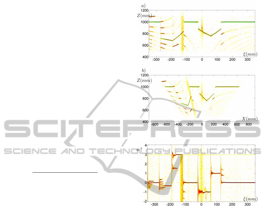
We conduct experiments to evaluate the proposed
Figure 5: Estimated depths.
Figure 6: Estimated slopes.
algorithm. Preliminary results are presented here.
The goal is to validate the algorithm. For that pur-
pose, the system is simulated with two test scenes.
The geometry of the first test scene is shown in fig-
ure 2. Parameters are as follows: camera: D
C
= 550,
∆ξ = 0.5, K = 1400, B = 1; projector: D
P
= 900,
∆η = 0.6, A = 1, T = 20∆η, σ
v
= 0.02. The algo-
rithm runs with N = 200 particles.
Figure 5 shows the resulting density estimate in
the Z,ξ domain, and in the X, Z domain. After each
transition, the particle filter produces a multimodal
distribution, but after a few steps, the curved solutions
die out. Within each continuity interval, the only sur-
vival is the true linear segment. Figure 6 shows the
resulting density of the slopes a
k
of these segments.
Within each continuity interval, the slope is first mul-
timodal, but after some steps it becomes unimodal.
Figure 7 shows the number of samples of each mode
for the first 120 steps. Most modes die out after 50
steps. These modes are the one that are most curved.
Two modes, however, are only slightly curved and die
after about 100 steps.
PARTICLE SMOOTHING FOR SOLVING AMBIGUITY PROBLEMS IN ONE-SHOT STRUCTURED LIGHT
SYSTEMS
535
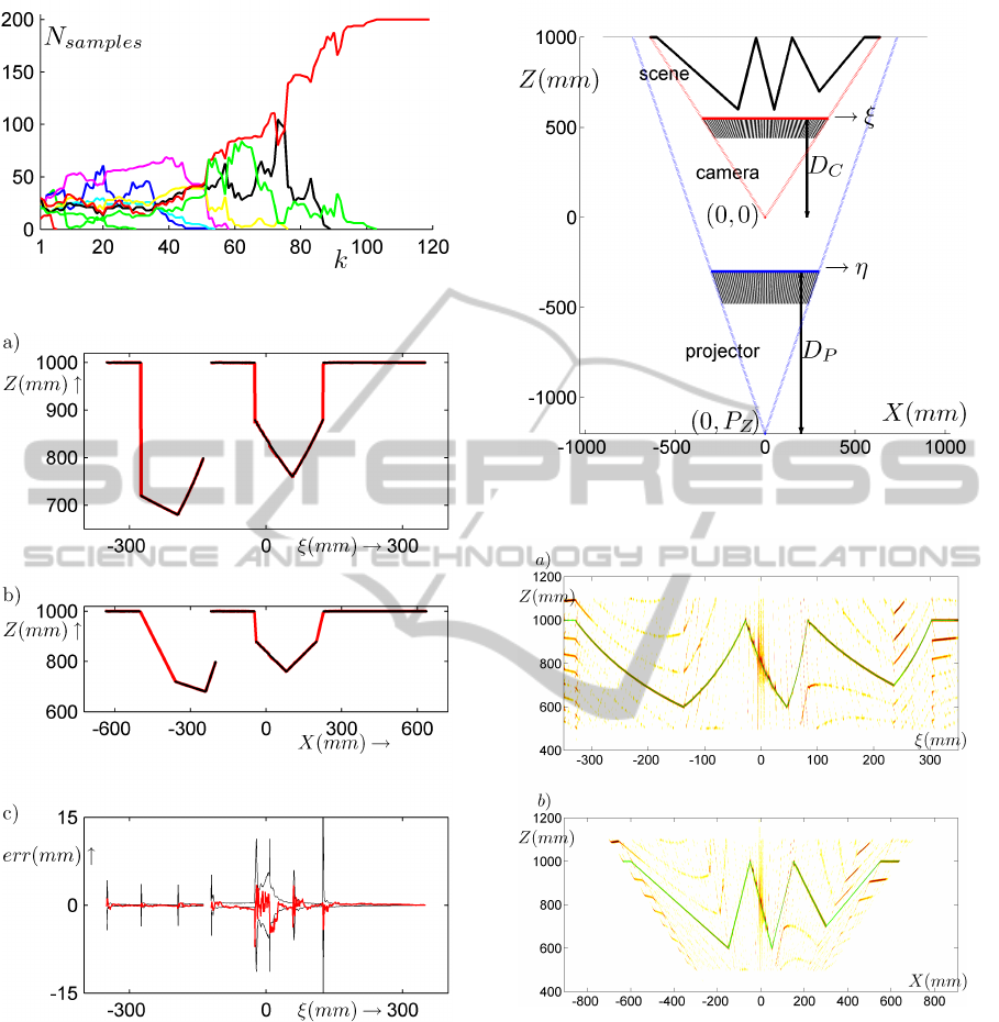
Figure 7: Nr. of samples/mode.
Figure 8: Results after particle smoothing. a) and b)
Smoothed estimates in the Z, ξ and the Z,X domain. Red
thick line = estimate; black thin lines = ground truth. c)
Estimation errors and indicated standard deviations.
We also observe in figure 5 and 6 that the lin-
ear segments are found faster if they are more in the
vicinity of the optical axis of the projector. This is
due to the fact that the ambiguous trajectories are
more curved near the optical axis, as shown in fig-
ure 4. At the optical axis, the measurement does not
provide any information about the depth. Yet, our
model driven particle filter provides an estimate there,
though at the cost of a larger noise sensitivity.
Figure 9: Test scene with walls that are near coplanar to the
viewing direction.
Figure 10: Particle filter depth estimates of the scene shown
in Figure 9.
The results after particle smoothing are presented
in Figure 8. The agreement between estimates and
ground truth is quite good. The ambiguities are re-
solved without errors. The profile exhibits 4 step
edges and 2 roof edges. All edges are detected cor-
rectly. There are no spurious edges. There is only
one localization error, which occurs at the roof edge
near ξ = 60. The cause can be traced back to the par-
ticle filter. The roof edge has discontinuities in the
derivatives, but the profile itself is continuous. Thus,
the measurements are only slowly running out of line
VISAPP 2011 - International Conference on Computer Vision Theory and Applications
536
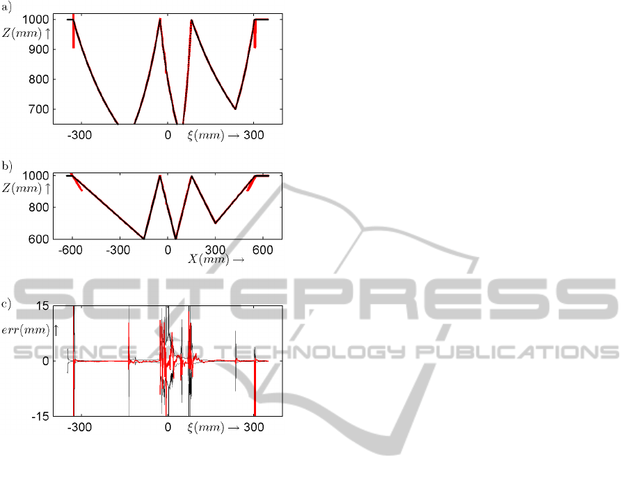
Figure 11: Results after smoothing.
with the currently estimated mode. Once a delay in
localization occurs, it cannot be undone by the back-
ward smoother because the smoother doesn’t rely on
measurements. The accuracy of the depth estimates
is depicted in Figure 8c. The standard deviation, ob-
tained from the EKF, is in line with the real estimation
errors. We observe that, scanning from left to right, at
each edge the standard deviation jumps to a higher
level, and then decays. The explanation is that our
smoother only selects particles, but it does not change
particles. Thus, a Kalman state, stored in a selected
particle, is not smoothed. Clearly, here some room
for improvement.
The test scene in Figure 2 contains one region that
is occluded. It can be observed in Figure 5 that the
particle filter produces a uniform probability density
in this area reflecting the fact that no information is
available in this region. During the smoothing pass
this region is removed from the map. This is eas-
ily accomplished since occlusions are reflected in the
measurements by an absence of a sinusoidal pattern.
We also tested the algorithm to a scene with ob-
jects whose main planes are near coplanar to the view-
ing direction. The scene is shown in Figure 9. The
imaging parameters are the same as in the first exam-
ple. The result of the particle filter and the smoother
are shown in Figure 10 and 11, respectively. Although
in these figures, the algorithm is successful (it finds
the correct solution), multiple runs of the algorithm,
with different random seeds, shows that this is not
always the case. Especially, in the left part of the
scene it may happen that the algorithm gets stuck in
the wrong mode. A possible explanation for this be-
haviour might be that the number of ambiguities on
the sides of the images is much larger than in the
central part. Moreover, all those solutions are near
linear. This is quite opposite to the central part. In
fact, on the optical axis of the projector the solution is
unique, and near the optical axis all spurious solutions
are highly curved.
7 CONCLUSIONS
This paper demonstrates that the ambiguity problem
in phase measuring profilometry can be solved if the
solution space is limited to polyhedral objects, and
if the geometrical set-up is suitably chosen. For that
purpose we have developed a new particle filter that
is inspired on jump Markov linear models. As a first
step, we have validated this design with a demon-
stration on simulated data. Currently we are con-
ducting additional experimentation on real data for a
more comprehensive evaluation with respect to accu-
racy and reproducibility.
REFERENCES
Arulampalam, M. S., Maskell, S., Gordon, N., and Clapp,
T. (2002). A tutorial on particle filters for online
nonlinear/non-gaussian bayesian tracking. 50(2):174–
188.
Doucet, A., Gordon, N. J., and Krishnamurthy, V. (2001).
Particle filters for state estimation of jump markov lin-
ear systems. 49(3):613–624.
Fong, W., Godsill, S. J., Doucet, A., and West, M. (2002).
Monte carlo smoothing with application to audio sig-
nal enhancement. 50(2):438–449.
Su, X. and Chen, W. (2001). Fourier transform profilom-
etry: A review. Optics and Lasers in Engineering,
35(5):263–284.
van der Heijden, F., Spreeuwers, L. J., and Nijmeijer, A. C.
(2009). One-shot 3d surface reconstruction from in-
stantaneous frequencies - solutions to ambiguity prob-
lems. In Int. Conf. on Computer Vision Theory and
Applications VISAPP2009, Lissabon. Visigrapp.
PARTICLE SMOOTHING FOR SOLVING AMBIGUITY PROBLEMS IN ONE-SHOT STRUCTURED LIGHT
SYSTEMS
537
