A CORTICAL FRAMEWORK FOR SCENE CATEGORISATION

. M. F. Rodrigues and J. M. H. du Buf

Institute for Systems and Robotics (ISR), Vision Laboratory

University of the Algarve (ISE and FCT), 8005-139 Faro, Portugal

Keywords:

Scene categorisation, Gist vision, Multiscale representation, Visual cortex.

Abstract:

Human observers can very rapidly and accurately categorise scenes. This is context or gist vision. In this paper

we present a biologically plausible scheme for gist vision which can be integrated into a complete cortical

vision architecture. The model is strictly bottom-up, employing state-of-the-art models for feature extractions.

It combines ﬁve cortical feature sets: multiscale lines and edges and their dominant orientations, the density of

multiscale keypoints, the number of consistent multiscale regions, dominant colours in the double-opponent

colour channels, and signiﬁcant saliency in covert attention regions. These feature sets are processed in a

hierarchical set of layers with grouping cells, which serve to characterise ﬁve image regions: left, right, top,

bottom and centre. Final scene classiﬁcation is obtained by a trained decision tree.

1 INTRODUCTION

Scene categorisation is one of the most difﬁcult is-

sues in computer vision. For the human visual system

it is quite trivial. We can extract the gist of an im-

age before we consciously know that there are certain

objects in the image, i.e., before perceptual and se-

mantic information is available which observers can

grasp within a glance of about 200 ms (Oliva and Tor-

ralba, 2006). Real-world scenes contain a wealth of

information whose perceptual availability has yet to

be explored. Categorisation of global properties is

performed signiﬁcantly faster (19 - 67 ms) than basic

object categorisation (Greene and Oliva, 2009). This

suggests that there exists a time during early visual

processing when a scene may be (sub-)classiﬁed as a

large open space or as a space with many regions etc.

We propose that scene gist involves two major

paths: (a) global gist, usually referred to as “gist,”

which is related more to global features (Ross and

Oliva, 2010), and (b) local object gist, which is able to

extract semantic object information and spatial layout

as fast as possible and also related to object segrega-

tion (Martins et al., 2009). Basically, local and global

gist are bottom-up processes that complement each

other. In scenes where there are (quasi-)geometric

shapes like squares, rectangles, triangles and circles

etc., local gist may “bootstrap” the system and feed

global gist for scene categorisation. This is predom-

inant in indoor scenes or man-made scenes. Exam-

ples include “ofﬁces” (indoor) with bookshelves and

computers, or “plazas” (outdoor) with trafﬁc signs

and facades of buildings. As explained by (Vogel

et al., 2007), humans rely on local, region-based in-

formation as much as on global, conﬁgural informa-

tion. Humans seem to integrate both types of informa-

tion, and the brain makes use of scenic information at

multiple scales for scene categorisation (Vogel et al.,

2006). In this paper we focus on global gist, simply

referred to as gist.

Concerning alternative approaches to global gist,

many include computations which are biologically

implausible. (Oliva and Torralba, 2006) used spectral

templates that correspond to global scene descriptors

such as roughness, openness and ruggedness. (Fei-

Fei and Perona, 2005) decomposed a scene into lo-

cal common luminance patches or textons. (Bosch

et al., 2009) applied SIFT, the Scale-Invariant Feature

Transform of (Lowe, 2004) to characterise a scene.

(Vogel et al., 2007) showed the effect of colour on the

categorisation performance of both human observers

and their computational model. In the ARTSCENE

neural system of (Grossberg and Huang, 2009), nat-

ural scene photographs are classiﬁed by using multi-

ple spatial scales to efﬁciently accumulate evidence

for gist and texture. This model embodies a coarse-

to-ﬁne texture-size ranking principle in which spatial

attention processes multiple scales of scenic infor-

mation, from global gist to local textures. Recently,

(Xiao et al., 2010) introduced the extensive Scene

UNderstanding (SUN) database that contains 899 cat-

egories and 130,000 images. From these they used

364

M. F. Rodrigues J. and M. H. du Buf J..

A CORTICAL FRAMEWORK FOR SCENE CATEGORISATION.

DOI: 10.5220/0003368603640371

In Proceedings of the International Conference on Computer Vision Theory and Applications (VISAPP-2011), pages 364-371

ISBN: 978-989-8425-47-8

 2011 SCITEPRESS (Science and Technology Publications, Lda.)

397 categories to evaluate various state-of-the-art al-

gorithms for scene categorisation and to compare the

results with human scene classiﬁcation performance.

In addition, they also studied a ﬁner-grained scene

representation in order to detect smaller scenes em-

bedded in larger scenes. In the Results section we

report some results of the methods mentioned above.

The rest of this paper is organised as follows. In

Section 2 we present the global gist model frame-

work, including the feature extraction and classiﬁca-

tion methods. In Section 3 we present results, and in

Section 4 a ﬁnal discussion.

2 GIST MODEL FRAMEWORK

Our gist model is based on ﬁve sets of features de-

rived from cells in cortical area V1: multiscale lines

and edges, multiscale keypoints, multiscale regions,

colour, and saliency for covert attention. These fea-

tures, which are explained in the following sections,

are combined in a data-driven, bottom-up process, us-

ing several layers of gating and grouping cells. These

cells gather properties of local image regions, which

are then used in a sort of decision tree, i.e., we do not

match any patterns but assume that the decision tree

is the result of a training process.

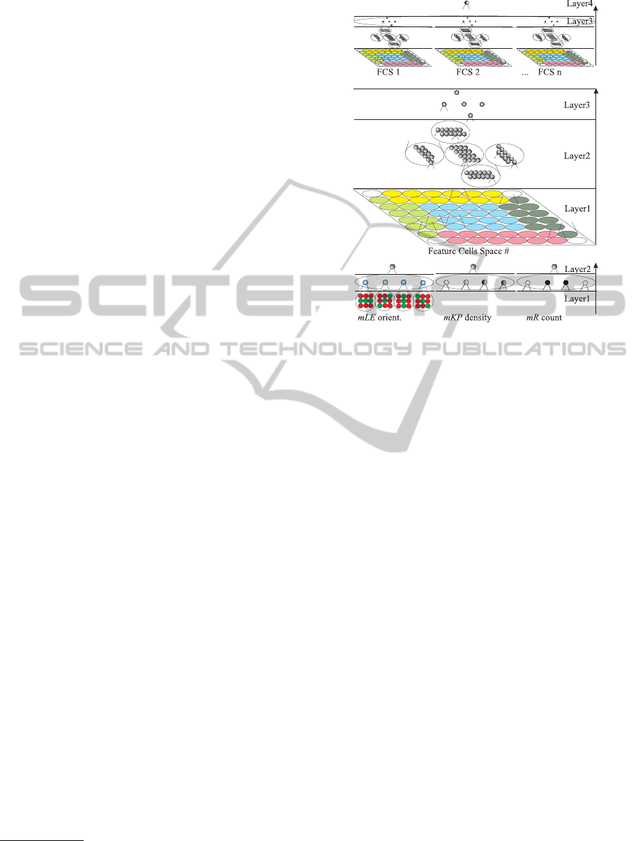
For each of the feature sets we apply a hierar-

chy of 4 layers of grouping cells with dendritic ﬁelds

(DFs). In the ﬁrst layer we have the feature space,

which is divided for the second layer into 8× 8 non-

overlapping DFs, for combining information within

each DF. The third layer combines information in left,

right, top, bottom and centre regions of the image in a

winner-takes-all manner. Figure 1 (middle) illustrates

how the 8 × 8 DFs are grouped into a 4 × 4 centre

region and the four neighbouring L/R/T/B regions of

10 (L/R) and 12 (T/B) DFs each, such that each DF is

only used once.

The fourth layer at the top implements a decision

tree on the basis of combinations of responses at layer

number three, using again the winner-takes-all strat-

egy, for classifying the scene; see Fig. 1 (top). Hence,

our gist framework combines ﬁve feature groups with

local-to-global feature extractions.

In our experiments we used the “spatialenvelope”

dataset which comprises colour images of 256× 256

pixels from 8 outdoor scene categories: coast, moun-

tain, forest, open country, street, inside city, tall build-

ings and highways

(Oliva and Torralba, 2001; Oliva

and Torralba, 2006). From this dataset we selected 5

Database available for download at:

http://people.csail.mit.edu/torralba/code/spatialenvelope/

Figure 1: The three layers for scene categorisation. Top:

global decision level. Middle: dendritic ﬁeld tree applied to

each feature in the input image. Bottom, left to right: group-

ing cells in layer 1 for detecting dominant orientations, key-

point density, and the number of regions in each DF. See

text for details.

categories: coast, forest, street, inside city and high-

way. This selection is a mixture of two man-made

scenes without signiﬁcant objects that could charac-

terise the scene (i.e., scenes in principle not bootable

by local gist), two natural scenes, and one scene that

combines (approx. 50%) natural (sky, trees, etc.) with

man-made aspects, the highways. Of each category

we randomly selected 30 images, a total of 150 im-

ages. One exception was the highway set, where im-

ages with salient cars were excluded because these

could be explored ﬁrst using local object gist.

The 150 images were split into two groups: 5 per

category for training (25) and 25 per category for test-

ing (125). Figure 2 shows in the leftmost column ex-

amples of the training set and in the other columns

examples of the test set.

2.1 Multiscale Lines and Edges

There is extensive evidence that the visual input is

processed at different spatial scales, from coarse to

ﬁne ones, and both psychophysicaland computational

studies have shown that different scales offer different

qualities of information (Bar, 2004; Oliva and Tor-

ralba, 2006).

We apply Gabor quadrature ﬁlters to model recep-

tive ﬁelds (RFs) of cortical simple cells (Rodrigues

A CORTICAL FRAMEWORK FOR SCENE CATEGORISATION

365

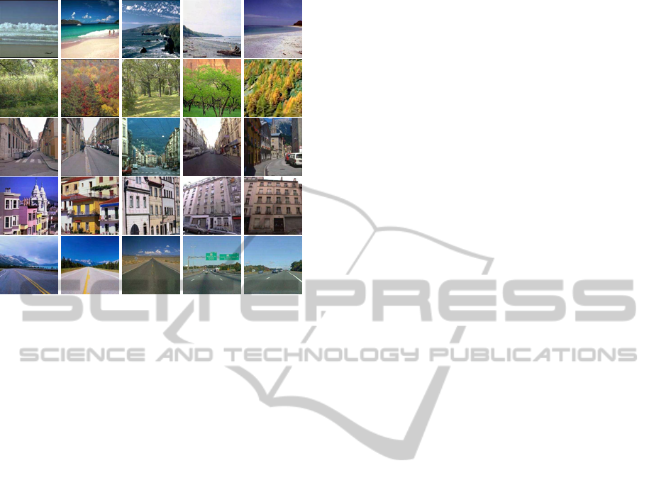
Figure 2: Examples of images of, top to bottom, coast, for-

est, street, inside city and highways. The left column shows

images of the training set.

and du Buf, 2006). In the spatial domain (x,y) they

consist of a real cosine and an imaginary sine, both

with a Gaussian envelope. The receptive ﬁelds (ﬁl-

ters) can be scaled and rotated. We apply 8 orienta-

tions θ and the scale of analysis s will be given by the

wavelength λ, expressed in pixels, where λ = 1 corre-

sponds to 1 pixel. All images have 256× 256 pixels.

Responses of even and odd simple cells (real and

imaginary parts of Gabor kernel) are obtained by con-

volving the input image with the RFs, and are denoted

by R

λ,θ

(x,y) and R

λ,θ

(x,y). Responses of complex

cells are then modelled by the modulus C

λ,θ

(x,y) =

[{R

λ,θ

(x,y)}

+ {R

λ,θ

(x,y)}

]

1/2

Basic line and edge detection is based on re-

sponses of simple cells: a positive (negative) line is

detected where R

shows a local maximum (mini-

mum) and R

shows a zero crossing. In the case

of edges, the even and odd responses are swapped.

This gives four possibilities for positive and negative

events. An improved scheme combines responses of

simple and complex cells, i.e., simple cells serve to

detect positions and event types, whereas complex

cells are used to increase the conﬁdence. Lateral and

cross-orientation inhibition are used to suppress spu-

rious cell responses beyond line and edge termina-

tions, and assemblies of grouping cells serve to im-

prove event continuity in the case of curved events.

For further details see (Rodrigues and du Buf, 2009b).

At each (x,y) in the multiscale line and edge event

space, four gating LE cells code the 4 event types

line+, line-, edge+ and edge-. These are necessary

for object recognition (Rodrigues and du Buf, 2009b).

Here in the case of gist we are only interested in bi-

nary event detection. This is achieved by a grouping

cell which is activated if a single LE gating cell is ex-

citated. In layer 1 (see Fig. 1) all events are summed

over the scales mLE =

∑

, with λ = [4,24] and

∆λ = 0.5, scale s = 1 corresponding to λ = 4. The

top-left image of Fig. 3 shows the result in the case of

the top-left image of Fig. 2.

Now, for each cell and DF in layer 1, we compute

the dominant orientation (horizontal, 45

, vertical and

135

) at each (x,y) in the accumulated mLE. This is

done using 4 sets of cell clusters of size 3 × 3. The

cell in the centre of a cluster is excitated if events are

present on the centre line. From the 4 clusters the

biggest response is selected (winner-takes-all). Fig-

ure 1 (bottom-left) illustrates the principle.

The same process is applied to all event cells mLE

in each DF, where similar orientations are summed

and the local dominant orientationis attributedto each

cell in layer 2 by the winner-takes-all strategy. This

process allows us to have different dominant orien-

tations (LE

) in different regions of the scene. For

instance, we expect that horizontal lines point more

to coastal scenes, vertical ones to buildings, diagonal

ones to streets, etc.

2.2 Multiscale Keypoints

Keypoints are based on end-stopped cells (Rodrigues

and du Buf, 2006). They provide important informa-

tion because they code local image complexity. There

are two types of end-stopped cells, single and double,

which are modelled by ﬁrst and second derivatives

of responses of complex cells. All end-stopped re-

sponses along straight lines and edges are suppressed,

for which tangential and radial inhibition schemes are

used. Keypoints are then detected by local maxima in

x and y. For a detailed explanation with illustrations

see (Rodrigues and du Buf, 2006).

At each (x,y) in the multiscale keypoint space,

keypoints are summed over the scales, mKP =

∑

, see Fig. 3 (1st row and 2nd column), using

the same scales as used in line and edge detection.

Again, for each DF all existing mKP are summed,

∑

mKP, resulting in a single value of all

keypoints present in each DF over all scales. This

value activates one of four gating cells that represent

increasing levels of activation (density of KPs) in each

DF in layer 1. Figure 1 (bottom-centre) illustrates the

principle. These gating cells activate the grouping cell

in layer 2 which codes the density of KPs.

Mathematically, the

are divided by the num-

ber of active KP cells at all scales in each DF re-

VISAPP 2011 - International Conference on Computer Vision Theory and Applications

366

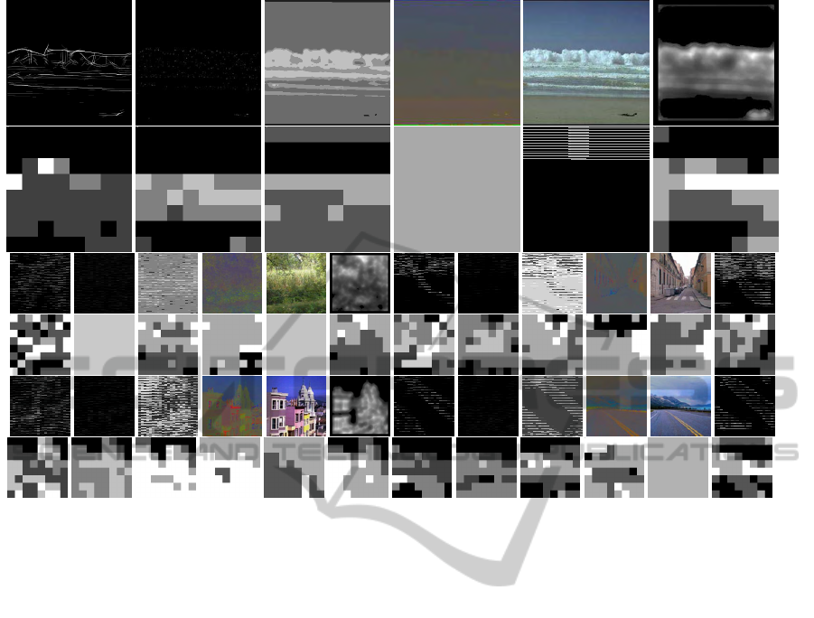
Figure 3: The odd rows show features in layer 1 of the images in the left column of Fig. 2. The even rows illustrate responses

of gating cells in layer 2, where the 8×8 array is represented by the squares. Gray level, from black to white, indicate response

levels A to D. See text for details.

gion, and the four intervals of the densities KP

the gating cells are [0, 0.01], ]0.01,0.1], ]0.1, 0.5] and

]0.5,1.0]. These values were determined empirically

after several tests using the training set.

2.3 Multiscale Region Classiﬁcation

As stated above, different spatial frequencies play dif-

ferent roles in fast scene categorisation, and low spa-

tial frequencies are thought to inﬂuence the detection

of scene layout (Bar, 2004; Oliva and Torralba, 2006).

To explore low spatial frequencies in combination

with different spatial layouts, we apply a multiscale

region classiﬁer. For creating four scales we itera-

tively apply a 3×3 averaging ﬁlter which increasingly

blurs the original image. Then, at each scale, we ap-

ply a basic region classiﬁer. The goal is to determine

how many consistent regions there are in each DF, as

this characterises the spatial layout. We only consider

a maximum of four graylevel clusters in each scene.

The basic region classiﬁer works as follows. Con-

sider 4 grouping cells with their DFs covering the en-

tire image. These cells cluster grayscale information

and are initially equally spaced between the minimum

and maximum levels of gray. In image processing ter-

minology, these cells represent the initial graylevel

centroids. The grayscale at each (x,y) in the image

is summed by the grouping cell which has the closest

centroid. When all (x,y) pixels have been assigned,

a higher layer of grouping cells is allocated. The

latter cells employ the mean activation levels of the

lower cells, i.e., they adapt the initial positions of the

4 centroids. This is repeated with 4 layers of group-

ing cells. Each pixel in the image is then assigned to

the closest grouping cell (centroid), which results in

an image segmentation.

The above process is applied to each scale inde-

pendently. Final regions are obtained by accumulat-

ing evidence at the four scales, mR. The ﬁnal value

at each (x,y) is the one that appears most often at the

different scales at the same position, but regions of

less than 4 pixels are ignored. If there is no domi-

nant value, when for example all scales at the same

(x,y) have different classes, the one from the coarsest

scale is selected. The dominant value is assigned to

the cells in layer 1, see Fig. 1 (bottom-middle). Fig-

ure 3 (1st row, 3rd column) shows the result.

For each DF in layer 1, four gating cells each

tuned to the 4 regions (clusters) in the image are ac-

tivated if those regions (labels) exist inside the DF.

Finally, the grouping cells in layer 2 code the number

of regions R

in the DF, by summing the number of

A CORTICAL FRAMEWORK FOR SCENE CATEGORISATION

367

activated gating cells. Figure 1 (bottom-right) illus-

trates gating cells by circles, with activated cells as

solid circles. In the speciﬁc case shown, two different

regions exist in this DF.

2.4 Colour

A very important feature is colour (Vogel et al., 2007).

We use the Lab colour space for two main reasons:

(a) it is an almost linear colour space and (b) we

want to use the information in the so-called double-

opponent colour blobs in area V1 (Tailor et al., 2000).

Red(magenta)-green is represented by channel a and

blue-yellow by channel b.

We process colour along two paths. In the ﬁrst

path we use corrected colours, because a same scene

will look different when illuminated by different light

sources, i.e., the number, power and spectra of these.

Let each pixel P

of image I(x, y) be deﬁned as

) in RGB colour space, with i = {1...N},

N being the total number of pixels in the image.

We process the input image using the two transfor-

mations described by (Martins et al., 2009), both in

RGB colour space. We apply iteratively steps A and

B, until colour convergence is achieved, usually af-

ter 5 iterations. Each individual pixel is ﬁrst cor-

rected in step A for illuminant geometry indepen-

dency, i.e., chromaticity. If S

= R

+ G

+ B

, then

= (R

). This is followed in step B

by global illuminant colour independency, i.e., gray-

world normalisation. If S

= (

∑

j=1

)/N with X ∈

{R,G,B}, then P

= (R

). After

this process is completed, see Fig. 3 (1st row, 4th col-

umn), the resulting RGB image is converted to Lab

colour space. For more details and illustrations see

(Martins et al., 2009). In the second path, the colour is

converted straight from RGB to Lab space; see Fig. 3

(1st row, 5th column).

The values of the two paths are assigned sepa-

rately to layer 1. There are 4 possible classes in

layer 2, represented by different grouping cells. Each

cell represents one dominant colour: red(magenta),

green, blue and yellow. For each pixel we com-

pute the dominant colour C

= max[max{|a

+ |,|a

−

|},max{|b

+ |,|b

− |}], and then the activation of the

grouping cell in layer 2 is determined by the dominant

colour in each DF,C

= max

{

∑

DF,a+

∑

DF,a−

∑

DF,b+

∑

DF,b−

}, with C

denoted by C

for

colour path one and by C

for colour path two.

2.5 Saliency

The saliency map S applied is based on covert atten-

tion. Here we use a simpliﬁed model which relies

on responses of complex cells, instead of keypoints

based on end-stopped cells (Rodrigues and du Buf,

2006), but it yields consistent results for gist vision.

A saliency map is obtained by applying a few

processing steps to the responses of complex cells,

at each individual scale and orientation, after which

results are combined: (a) Responses C

λ,θ

(x,y) are

smoothed using an adaptive DOG ﬁlter, see (Martins

et al., 2009) for details, obtaining

λ,θ

. (b) The results

at all scales and orientations are summed, S(x,y) =

∑

λ,θ

(x,y). (c) All responses below a threshold of

0.1· maxS(x,y) are suppressed. This saliency map is

available in the feature space in layer 1, see Fig. 3 (1st

row, 6th column).

For computation purposes, the saliency in the

scene is coded from 0 to 1, where 0 means no saliency

and 1 the highest level of saliency possible. One of

four gating cells at each position can be activated ac-

cording to the level of saliency S

: the intervals are

[0,0.25[, [0.25,0.5[, [0.5,0.75[ and [0.75,1]. For each

DF, 4 grouping cells sum the number of activated gat-

ing cells representing the four levels and, by winner-

takes-all, the dominant saliency level in each DF is

selected and assigned to the grouping cell in layer 2.

The odd rows in Fig. 3 show the feature spaces at

layer 1, in the case of the images shown in the leftmost

column, from top to bottom, in Fig. 2. The 5 features

are, from left to right: lines/edges, keypoints, regions,

normalised colour, original colour, and saliency. The

even rows illustrate responses of the 8 × 8 grouping

cells in layer 2, each represented by a square. The four

activation levels of each feature dimension are repre-

sented by levels of gray, from black to white. Below

these are named A to D.

2.6 Scene Classiﬁcation

The above process can be summarised as follows:

(a) compute the features: multiscale lines and edges

(LE

), multiscale keypoints (KP

), multiscale regions

¯s

), colour (C) and covert attention saliency (S). (b)

Divide the image in 8× 8 dendritic ﬁelds (DFs). (c)

For each DF in layer 1 apply the following steps:

(c.1) for LE

, sum all events at all scales mLE, and

compute the dominant orientations. Each grouping

cell in layer 2 is coded as LE

= {A = 0

;B =

;C = 90

;D = 135

(c.2) Sum KP

over the scales, and over

the DF

, and compute the density.

Each grouping cell in layer 2 is coded as

= {A ≤ 0.01(very low);B ∈]0.01,0.1](low);C ∈

]0.1,0.5](medium);D > 0.5(high)}.

(c.3) Compute the accumulated evidence of regions

mR, and count in each DF the number of regions:

VISAPP 2011 - International Conference on Computer Vision Theory and Applications

368

= {A = 1;B = 2;C = 3;D = 4}.

c.4) Compute the colour-opponentdominant colourC

at each position and then over the DFC

in Lab colour

space. Grouping cells in layer 2 code the dominant

colour of normalised and original colours C

dn/dc

{A = a+;B = a−;C = b+;D = b−}.

(c.5) Compute the saliency level: each grouping cell

in layer 2 is coded by S

= {A ∈ [0,0.25](very low);

B ∈]0.25,0.5](low); C ∈]0.25, 0.5](medium); D ∈

]0.75,1](high)}.

Finally, (c.6) apply winner-takes-all to each of the

above classiﬁcations. In layer 2 each image is coded

by clusters of 6 grouping cells (LE

, KP

, R

, C

and S

) times the number of cells with DFs in the

layer, 8× 8 = 64.

To classify the scenes, we accumulate evidence of

each feature in ﬁve image regions: Top, Bottom, Left,

Right and Centre; see Fig. 1, middle layer 2. As men-

tioned before, all clusters of feature cells in T, B, L,

R and C are summed by grouping cells in layer 3. In

top layer 4, the features in the regions are combined

for ﬁnal scene classiﬁcation.

In layer 3 only the most signiﬁcant responses from

layer 2 are used, i.e., (a) for each feature and region

we extract, using 4 grouping cells, the sums (his-

tograms) of the different feature codes A to D, and (b)

by winner-takes-all we select the most frequent code.

A grouping cell in layer 3 is only activated if (c) this

code is present in at least half of the DFs of each re-

gion in layer 2: these are 16/2 = 8 in C, 12/2 = 6 in

T/B and 10/2 = 5 in L/R.

There are three exceptions concerning LE

, KP

and S

, when no code ﬁts condition (c). In these cases

a cell “no response” is activated, coded by N from No.

As a result, in layer 3 we have the following clusters

of cells: 6 features times 5 regions times 4 (A-D) or

5 (A-D plus N). Figure 4 shows them in the case of

a coast (left) and forest (right), the top two images in

the left column of Fig. 2.

At layer 4 there are only ﬁve cells which code the

type of the input scene, from coast to highway. Be-

tween layer 3 and layer 4 there are four sub-layers of

gating and grouping cells which combine evidence for

scene-speciﬁc characteristics. These sub-layers were

trained by using the responses of the 5 training im-

ages of each class. The idea is that at the start each

input scene can trigger several classes but in higher

sub-layers the number of classes is reduced until only

one remains. It is also possible that only one class

remains at a lower sub-layer, in which case the clas-

siﬁcation can terminate at that sub-layer and the class

passes directly to layer 4. This is a type of decision

tree with levels numbered from 3.i to 3.iv:

Sub-layer 3.i: Gating cells act as ﬁlters on the regions

L/R/T/B/C separately, and their outputs are summed

together, i.e., only the dominant code is important.

These ﬁlters are shown in column i in Tab. 1. For ex-

ample, in the case of a coast scene, dominant lines and

edges must be horizontal (A) or absent (N), keypoint

density may not be high (not D), the dominant colours

of the non-normalised image must be A (a+=red), C

(b+=blue) or D (b-=yellow), and saliency may not

be high (not D) nor not present (not N). For coast

scenes the region and normalised colour features are

excluded. Different ﬁlters are applied for all scene

types.

Sub-layer 3.ii: Similar to the previous level, new ﬁl-

ters are applied at level ii. The outputs of different

regions of level i are ﬁrst ORed together: left/right

(LR) and top/centre/bottom (TCB). In the case of a

coast scene, see column ii in Tab. 1, an input scene

can only pass level ii if at least one combination (LR

and/or TCB) satisﬁes the line/edge orientations, key-

point densities and original colours. An “e” in column

ii (forest, highway) indicates the AND operator, i.e.,

a forest scene must have a medium (C) or high (D)

keypoint density in LR as well as in TCB.

Sub-layer 3.iii: The “e” and “z” in column iii in Tab.1

stand for excitated and zero, respectively. These are

ANDed together. Looking again at the coast case:

a scene must have horizontal lines/edges in LR and

TCB, but no vertical ones, and saliency may not be

high.

Sub-layer 3.iv: At this level a scene class must be at-

tributed. For this reason the OR and AND operators

are not used but the SUM operator, such that different

feature combinations of the classes can lead to one

maximum value which deﬁnes the class. Column iv

in Tab. 1 lists the feature combinations. A “+” means

that a feature cell (at least one in the L/R/T/C/B re-

gions) must be activated, and counts for 1 in the sum.

A “0” means that a feature cell must not be activated.

If not activated it also counts for 1, but if activated

it contributes 0 to the sum. In all ﬁve classes, the

maximum sum is 8. If there is still an image with

two scene classiﬁcations with the same sum, the same

classiﬁcation principle as applied in this sub-layer is

now applied to all the cells in layer 2 (the sum of all

cells that meet the criteria).

3 RESULTS

The training set of 5 images per scene resulted in a

recognition rate of 100%, because the decision tree

was optimised by using these. On the test set of 25

images per scene, with a total of 125 images, the total

recognition rate was 79%; for each class: coast 84%,

A CORTICAL FRAMEWORK FOR SCENE CATEGORISATION

369

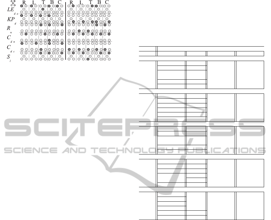
Figure 4: Cell clusters in layer 3 with activated cells shown

dark; coast (left) and forest (right).

forest 96%, street 72%, inside city 76% and highways

64%. Table 2 presents the confusion matrix. As men-

tioned in the Introduction, gist vision is expected to

perform better in case of natural scenes, coasts and

forests, and this is conﬁrmed by a combined result of

90%. In case of man-made scenes, street and inside

city, the combined result is 84%. Here we expected

a lower performance due to increased inﬂuence of lo-

cal object gist related to the many geometric shapes

which may appear in the scenes.

Highways gave an unexpected result. We ex-

pected a rate between the rates of natural and man-

made scenes. In Tab. 2 we can see that some high-

ways were classiﬁed as streets, probably because

wide streets are quite similar to narrow highways.

However, most misclassiﬁed highways ended up as

coasts, which means that the feature combinations

must be improved. Looking into more detail, and re-

lated to the suggestions of (Greene and Oliva, 2009),

there exists a time during early visual processing

where a scene may be classiﬁed as, for example, a

“large space or navigable, but not yet as a mountain

or lake.” Both highways and coasts may have clouds

and blue sky at the top, a more or less prominent hori-

zon line in the centre, and at the bottom a more or less

open space. This suggests that the method can detect

these initial characteristics, but not yet discriminate

enough between the two classes. An additional test in

which these two categories were combined for detect-

ing “large open spaces with a horizon line” yielded a

recognition rate of 86%.

In Tab. 2 we see that 12% of street images and

16% of inside city images were labelled as “no class.”

This is due to the images not obeying the criteria of

sub-layers 3.i to 3.iii. Again, these were images with

man-made objects. Inspection of the unclassiﬁed im-

ages revealed that most of them contain a huge num-

ber of geometric shapes like windows, which is an

indication for the role of local object gist vision based

on low-level geometry (Martins et al., 2009).

We can compare our results with those of other

studies in which the same dataset has been used.

Table 1: Response combinations at layer 3, sub-layers (i) to

(iv). The symbol “o” represents activated cells in the feature

cluster which are summed in layer i but combined by OR

in layer ii. The symbols “e” and “z” stand for excitated and

zero. In layer iii cell outputs are combined by AND. In layer

iv, cells are summed (counted), combining both active cells

“+” and not active cells “0” at the corresponding positions.

sub-layer i ii iii iv

cell A B C D N LR TCB A B C D N A B C D N

coast

o o o o e z + 0 0

o o o o o 0

o o o o o

o o o z + 0

forest

o o o z 0

o o e e z z 0 0

o o o z 0

o o o o z e +

o o o o 0 0

o o 0

street

z 0 0

o o o o 0 +

e 0 +

o o o o o +

o o o o o 0

inside city

o o o o z e 0 +

o o o 0

o o +

o o 0

o o 0 +

highways

z 0

o o 0 0

o o o

o o o e +

o o o e e e 0 +

o o o z + 0

(Oliva and Torralba, 2001) tested 1500 images of the

four scenes coast, country, forest and mountain, with

an overall recognition rate of 89%. A test of the four

scenes highway, street, close-up and tall building also

yielded a rate of 89%. (Fei-Fei and Perona, 2005)

tested 3700 images of 13 categories, with 9 natural

scenes of the same dataset that we used plus 4 oth-

ers (bedroom, kitchen, living room and ofﬁce), and

obtained a rate of 64%. (Bosch et al., 2009) tested

3 datasets. The best performance of 87% was ob-

tained on 2688 images of 8 categories. (Grossberg

and Huang, 2009) tested the ARTSCENE model on

1472 images of the 4 landscape categories coast, for-

est, mountain and countryside, and they achieved a

rate of 92%. Hence, our own result of 79% on 5 cat-

egories can be considered as good. Of all methods,

our own and the ARTSCENE models are the only bi-

ologically inspired ones. On natural scenes both mod-

els performed equally well: ARTSCENE gave 92% in

the case of 4 scenes and our model gave 90% on the 2

scenes coast and forest.

VISAPP 2011 - International Conference on Computer Vision Theory and Applications

370

Table 2: Confusion matrix of classiﬁcation results. Main

diagonal: correct rate. Off diagonal: misclassiﬁcation rates.

79% coast forest street in. city highways no class

coast 84% 16%

forest 96% 4%

street 72% 12% 4% 12%

in. city 8% 76% 16%

highways 24% 12% 64%

4 DISCUSSION

In this paper we presented a biologically plausible

scheme for gist vision or scene categorisation. The

model proposed is strictly bottom-up and data-driven,

employing state-of-the-art cortical models for feature

extractions. Scene classiﬁcation is achieved by a hi-

erarchy of grouping and gating cells with dendritic

ﬁelds, with local to global processing, also imple-

menting a sort of decision tree at the highest cell

level. The proposed scheme can be used to bootstrap

the process of object categorisation and recognition,

in which the same multi-scale cortical features are

employed (Rodrigues and du Buf, 2009a). This can

be done by biasing scene-typical objects in memory,

likely in concert with local gist vision and spatial lay-

out, i.e., which types of objects are about where in the

scene, but driven by attention. Although our model

of global gist does not yet yield perfect results, it is

already possible to combine it with a model of local

gist which addresses geometric shapes (Martins et al.,

2009).

In the future we have to increase the number of

test images and scene categories. This poses a prac-

tical problem because of the CPU time involved in

computing all multiscale features. This problem is be-

ing solved by re-implementing the feature extractions

using GP-GPUs.

ACKNOWLEDGEMENTS

Research supported by the Portuguese Foundation

for Science and Technology (FCT), through the

pluri-annual funding of the Inst. for Systems and

Robotics (ISR/IST) through the POS

Conhecimento

Program which includes FEDER funds, and by the

FCT project SmartVision: active vision for the blind

(PTDC/EIA/73633/2006).

REFERENCES

Bar, M. (2004). Visual objects in context. Nature Rev.:

Neuroscience, 5:619–629.

Bosch, A., Zisserman, A., and Munoz, X. (2009). Scene

classiﬁcation via pLSA. Proc. Europ. Conf. on Com-

puter Vision, 4:517–530.

Fei-Fei, L. and Perona, P. (2005). A Bayesian hierarchi-

cal model for learning natural scene categories. Proc.

IEEE Comp. Vis. Patt. Recogn., 2:524–531.

Greene, M. and Oliva, A. (2009). The briefest of glances:

the time course of natural scene understanding. Cog-

nitive Psychology, 20(4):137–179.

Grossberg, S. and Huang, T. (2009). Artscene: A neural

system for natural scene classiﬁcation. Journal of Vi-

sion, 9(4):1–19.

Lowe, D. (2004). Distinctive image features from scale-

invariant keypoints. Int. J. Comp. Vision, 2(60):91–

110.

Martins, J., Rodrigues, J., and du Buf, J. (2009). Focus of

attention and region segregation by low-level geome-

try. Proc. Int. Conf. on Computer Vision Theory and

Applications, Lisbon, Portugal, Feb. 5-8, 2:267–272.

Oliva, A. and Torralba, A. (2001). Modeling the shape of

the scene: a holistic representation of the spatial enve-

lope. Int. J. of Computer Vision, 42(3):145175.

Oliva, A. and Torralba, A. (2006). Building the gist of a

scene: the role of global image features in recognition.

Progress in Brain Res.: Visual Perception, 155:23–26.

Rodrigues, J. and du Buf, J. (2006). Multi-scale keypoints

in V1 and beyond: object segregation, scale selection,

saliency maps and face detection. BioSystems, 2:75–

90.

Rodrigues, J. and du Buf, J. (2009a). A cortical frame-

work for invariant object categorization and recogni-

tion. Cognitive Processing, 10(3):243–261.

Rodrigues, J. and du Buf, J. (2009b). Multi-scale lines and

edges in v1 and beyond: brightness, object categoriza-

tion and recognition, and consciousness. BioSystems,

95:206–226.

Ross, M. and Oliva, A. (2010). Estimating perception of

scene layout properties from global image features.

Journal of Vision, 10(1):1–25.

Tailor, D., Finkel, L., and Buchsbaum, G. (2000). Color-

opponent receptive ﬁelds derived from independent

component analysis of natural images. Vision Re-

search, 40(19):2671–2676.

Vogel, J., Schwaninger, A., Wallraven, C., and B¨ulthoff, H.

(2006). Categorization of natural scenes: Local vs.

global information. Proc. 3rd Symp. on Applied Per-

ception in Graphics and Visualization, 153:33–40.

Vogel, J., Schwaninger, A., Wallraven, C., and B¨ulthoff, H.

(2007). Categorization of natural scenes: Local versus

global information and the role of color. ACM Trans.

Appl. Perception, 4(3):1–21.

Xiao, J., Hayes, J., Ehinger, K., Oliva, A., and Torralba, A.

(2010). Sun database: Large-scale scene recognition

from abbey to zoo. Proc. 23rd IEEE Conf. on Com-

puter Vision and Pattern Recognition, San Francisco,

USA, pages 3485 – 3492.

A CORTICAL FRAMEWORK FOR SCENE CATEGORISATION

371